JoSS Article: Volume 4

Also availible as a .pdf here

Exploring the Dynamics of International Trade by Combining the Comparative Advantages of Multivariate Statistics and Network Visualizations

Lothar Krempel¹ and Thomas Plümper²

Abstract

This paper contributes to an ongoing debate in International Political Economy about the appropriateness of globalization, regionalization and macroeconomic imbalance theory by identifying quantitative estimates for all three tendencies from world trade data. This is achieved with a series of gravity models enhanced stepwise by the mapping of the estimation errors of a given model on representations of the overall structure of trade. This not only allows the identification of imperfections in a given model but also permits the further improvement of the models since any systematic regional organization in the error-terms can be identified. The results of the most elaborated model indicate that single factor explanations of global economic integration are presumably misleading. Instead, each of three explanations captures only part of the ongoing changes, as they can be identified under a comparative static perspective from world trade data.

1 Introduction

There is little doubt that multivariate regression analysis is among the most appropriate tools to test hypotheses if sufficiently reliable data is available. During the last decades, statistical analysis has been refined and an ever growing set of statistical tests and sophisticated approaches enable the researcher to cope with all kinds of ambiguities in the analyzed data sets (Beck & Katz 1995; Cramer 1986; White 1980). Crucial for obtaining valid parameter-estimates with regressions is the degree to which the common assumptions of regression analysis are met, especially that of the independence of the error terms and whether these latter have the same variance. While statistical analysis provides tests to check if a given model meets these assumptions, these tests are not very instructive on how to improve the model when the assumptions are hurt.

To cope with these problems within the research process we suggest extending the researcher's toolkit by a second technology. Tools for visualizing social structures can improve the specification of a given model if there is structure in the error terms. These visualizations allow the researcher to monitor the spatial organization of the resulting estimation errors and guide him or her in the process of improving the accuracy of the parameter estimates. In this article we will show how the visualization of the overall structure of world trade provides a very useful tool to enhance and analyze gravity models.

The problem of international trade analyzed in this paper can be considered as fairly typical for the use of quantitative estimates. Crude estimates for trends in economic processes can be obtained by comparing parameter estimates cross-sectionally and between different points in time. The ratio of corresponding estimates provides an insight into the dynamics of international economic activities. Furthermore, since the internationalization of economic activities can easily be measured by an analysis of the bilateral trade flows between countries, the widely acknowledged standard problem of social research the small-N problem does not occur. This is where network visualization tools can help.

The fruitfulness of the interplay of both technologies for that purpose is based on the fact that both extract different kinds of information usually given by gravity models. While statistical tools treat flows as independent units, visualizations can make use of any relational information pertaining to the pairs as they are used for the regression analysis. Visualizations provide the researcher with a view of the overall system. Our purpose here is twofold. First, we link statistical analyses and visualization techniques and use both tools in parallel for a stepwise improvement of gravity models. Second, we apply the method to the analysis of international economic processes, showing that concepts aimed at the explanation of global economic processes grasp just certain aspects of these processes. We conclude, therefore, that economic integration is best studied by a mixture of seemingly competing theories.

2 Specifying the Model by Stepwise Approximation

In this section we develop a baseline gravity model. The estimates we present here are based on bilateral trade between the 30 (26) biggest trading nations in 1994³. In the comparative static extension of this model in the section 3, the number of countries is widened to 45 countries. Furthermore, we present some evidence by comparing the estimates for the fifteen years between 1980 and 1994.

A commonly accepted method to inspect the factors influencing trade flows within a set of countries is to perform a regression analysis on the volume of all trade flows occurring between these countries.

This implies that the flows between different countries are independent from each other⁴. Even though this assumption is certainly not completely beyond criticism, economists are still willing to accept it. As we have emphasized earlier, a sufficient model in technical terms is not just characterized by the amount of explained variance. Any parameter estimates are only valid in the absence of systematic errors. The tool employed to detect systematic error components is the mapping of the residuals on the overall geographical structure of trade.

2.1 Network and Information Visualization

In an earlier paper (Krempel & Plümper, 1999) we have shown that the information contained in the trade data (the trade volumes) can be used to reconstruct the overall pattern of global trade visually, and that these images are a very useful basis for the evaluation of specific internationally occurring phenomena.

The key idea of such a graphical technology is to treat trade data as a valued graph in which the countries are considered to be the nodes and are linked by trade flows. This information can be ordered in various ways.

Such drawings can be further enriched if additional external data (attributes) are available for the system. In such a case it is possible to map this external information with color schemes onto the layout. This can help to identify local concentrations of such attributes for specific positions.

Mapping the residuals of a given statistical model with corresponding color schemes onto graph layouts allows the ability to locate systematic patterns. Consequently, using such visualizations supplies the researcher with additional information, since it is difficult to retrieve this particular supplementary information from the outcomes of statistical procedures by itself.

Our interest in this paper is to simultaneously inspect geographical distance, the volumes of trade and the accuracy of the trade estimates. A visualization should allow for the location of trade in geographical space, the visualization of the volume of flows, and the total exports and imports of the countries represented by symbols of different size. The accuracy of the estimates can be mapped with a color scheme onto the trade symbols.

For our purpose, a schematic placement of the countries seems to be most appropriate, for which we use the grand-circle distances between the country capitals.⁵ To enhance the amount of information that can be communicated with two-dimensional maps, we try to simplify geographical space with automatic layout routines. These transform the metric information into a simplified topology. While topologies sacrifice some of the metric distance information, they can preserve the general appearance of geographical space. Their optimized spacing allows for further communication of trade volumes using symbols of different size. For an inspection of how estimation errors are related to geographic space, any arrangement which does not change the neighborhoods of the geographic locations is sufficient: neighbors or neighborhoods which show similar colors (deviations) point to a local or regional organization of the error terms.

The embedding which we use to display the trade data has been computed with a spring embedder from the geographic distances and we use a straight-line representation of the trade flows. Spring embedders are a family of flexible algorithms that can order binary and valued graphs (Eades 1984, Kamada & Kawai 1989, Fruchterman & Reingold 1991). For an overview, see Brandes (1999, 2001), extensions for valued and two-mode graphs are discussed in Krempel (1999). Spring embedders can shrink long distances and spread dense centers of metric layouts so that the neighborhoods in the drawing are not changed.

Kamada & Kawai's algorithm is a multi-dimensional scaling algorithm (MDS) which uses a special local optimization function and is appropriate to order network data that are distances. Weighted versions of Fruchterman and Reingold's algorithm can produce topologies in which the spacing of the nodes (the image distances) can be optimized by tuning repulsive forces. This algorithm can thus be used as a tool in which to transform metric distances into topologies. The schematic map that we use in this paper has been produced with the latter algorithm. The image positions and their distances are still relatively strongly related to the data distances, being computed from the latitudes and longitudes of the country capitals (Pearson r=.9452).

This simplified map allows the rendering of all bilateral trade flows with arrows of corresponding size onto the layout. The volume of flows is symbolized by the size of the arrows linking any two nodes in the image. In order to link the visual approach to the statistical analysis, we use the size of the flows to inform us about the volumes of trade and their colors to inform us about the accuracy of the estimates. Treating the error terms as attributes of the flows and to transfer these with a color scheme onto the layout allows not only the inspection of misrepresented trade with a given model but also to visually identify how estimation errors are linked to the volume of the flows.

The complete information, of how the imports and exports of a specific country are misrepresented by a given model, can be read from the color distributions of the pie-charts, which represent the total of the imports (top) or exports (bottom) of a country.

This approach allows for the detection of neighborhoods that are strongly misrepresented by a specific model. As many of the trade flows still overlap even in the simplified map, we additionally supply interactive versions of the images. They take advantage of the capabilities of Scalable Vector Graphics (SVG) and allow for the exploration of the trade flows interactively by the accuracy of their estimates and by the origins and destinations of the shipments.

By mapping the error terms we not only evaluate the model's fit but also try to show what is not captured by a given model. The visualization of the errors reveals any systematic organization in the unexplained variance that is distance or neighborhood related. We have stressed before that any well fitting model implies a random distribution of the error terms. Thus, it is of special interest if we find any coherent color pattern when mapping the errors of a specific model onto the visualizations of the trade flows. Hence, any such pattern identified is an indicator of the insufficiency of a model; the assumption of the randomness of the error terms thereby being clearly violated.

This visual approach has several advantages compared to other ways of evaluating the model's accuracy. Contrary to classical statistical procedures that try to validate the model assumptions by testing for heteroskedasticity and autocorrelation (Hanushek & Jackson 1977, Wonnacott & Wonnacott 1979), the visualizations of the errors not only give evidence about the insufficiency of a model, but also help to locate where, and to which degree, single countries constitute exceptions that are not captured with a specific model. In other words, this procedure helps us to eliminate the sources of heteroskedasticity and autocorrelation instead of just circumventing its consequences as White-corrected standard errors (White 1980) or similar procedures do.

Whether a given trade flow is misrepresented can easily be inspected visually. If flow estimates of a given dyad are false, the connecting arrow for this flow is colored accordingly. To capture stronger distortions visually, we use different degrees of deviation of the estimated trade value from the observed. The information that we gathered in the arrows is aggregated to country information in the nodes. Nodes symbolize the total of the imports and the exports by the degree to which parts or even all of a country's trade is deviating from the estimates of a given model. The degree to which a specific country is consistently over- or underestimated can easily be read from the country symbols used in the visualizations. In the aggregate, systematic estimation errors for even larger regions should appear as similarly colored clusters in the visualizations. Areas of large standard errors point to geographic imperfections of a given model.

Moreover, functional imperfections of a given model can also be detected if the researcher has a good working hypothesis about a possible correlation between two functional variables. We will later show that a loose economic tie between nations belonging to the British Commonwealth of Nations still exists. Trade between two Commonwealth Nations is positively influenced by political, cultural or economic links, or if one is unwilling to accept that cultural factors determine this effect one may think in terms of an easing of business activity due to a common language.

Supplementing the statistical modeling efforts with the above described visualizations does not only provide useful information about the appropriateness of a model but also makes it easier to think of additional factors. We, stepwise, include detected variables to enhance the model and its prediction. After a series of such refinements and enhancements we proceed to the final step of our analysis where we introduce dummy variables for the different regions of world trade and turn to a larger sample of countries to test the robustness of our findings and to analyze the international economic dynamics under a comparative static perspective. The estimates for these regions obtained in the last step can be understood to give a comparative characterization of the preferences for regional trade in absence of distance, size of GDP and maritime transportation, joint borders etc.

2.2 Improving the Gravity Model by 'Eye-Balling'

Figure 1: Residuals Model 1

The node symbols allow for the reading of the extent to which the national imports (top) and exports (bottom) are misrepresented with a given model.

Use the following links to access two SVG versions of this graphic to explore the image interactively by the accuracy of flow estimates m1quality.html and by the origin and destination of trade m1country.html .

The basis of our analysis is a selection of the 26 biggest countries as traders in the world trade and their bilateral (asymmetric) trade in 1994. The dependent variable is the log of the values of goods traded from country i to country j. As open economies differ from closed economies due to the fact that they can borrow resources from the rest of world or lend them abroad (Obstfeld & Rogoff 1996), trade flows from i to j are not necessarily identical to the value of the flow from j to i. The most simple model uses the distance between the trading partners as a proxy for transportation costs. While the transportation cost is only one component of the overall transaction cost (tariffs and non-tariff barriers to trade, communication costs, market entry costs, information collection costs etc.), it is nevertheless the best single indicator available and should to a certain extent reflect any changes in world trade stemming from an increasing internationalization. The degree of economic internationalization can best be estimated by starting with a simple model. The first and most simple model tries to explain the trade flows between all countries by their geographical distance. In this first iteration of 'stepwise approximation' we use the (log) distance as a single explaining variable for all countries. Geographic distance is a crude but very basic indicator for transportation cost. Hence, we estimate:

log(TRD_ij) = a+DIST_ij^b+u_ij

where TRD_ij is the amount of trade from country i to country j in $US and DIST_ij the distance between the capitals of i and j in miles. Furthermore, we use the log of distance as a first independent variable. With increasing geographical distance the volume of trade should decrease. The choice of the logarithm of the distances is consistent with the fact that transport is a combination of fixed and variable cost. The loading and unloading of freight is more costly than the actual transport. Choosing the log distance as a proxy for the variable cost reflects the diminishing increase of the variable cost with long distance transport according to the 'iceberg model' of economic geography (Krugman 1998).

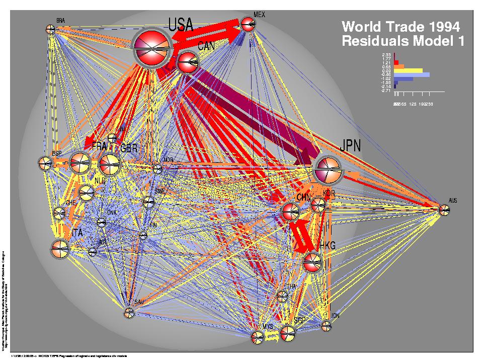
The distances used for our analysis are based on the location of the capitals of all countries and are computed as the grand circle distances. Even though these distances are a fair indicator for the transportation costs of distant countries, they do not appear to be completely without problems. Problematic are dyads consisting of neighboring countries or dyads in which the capital of at least one of the countries is strongly dislocated from the country's geographical center. If both conditions are present, we expect a crucial underestimation of real trade by the model. This is the case for Hong Kong and China (Beijing) where most of the trade takes place between Hong Kong and the southern provinces of China. Using the geographical distance as a single independent variable in our first model, we find an explained variance of 17 percent in 1994. The negative estimate for b = -.8274 indicates that distance and transportation costs still matter in the world trade of 1994.

A closer look at the visualization of the errors reveals, especially, that the large trade flows are heavily underestimated in this model. For the large traders symbolized with the size of their spheres, respectively the pies for their total imports (top) and exports (bottom) we find that almost all of their trade is underestimated: large countries trade more than can be estimated with the knowledge of the distance of their trading partners.

The reverse is true for small countries. Model 2 corrects this wrong specification be introducing country size into the model. We additionally take the GDP of both trading partners into account.

log(TRD_ij) = a+DIST_ij^b+GDP_i^c+GDP_j^d+u_ij

Such a model usually creates the core of a gravity model: "Flows in human geography are often termed spatial interactions, and a spatial interaction model is an equation that predicts the size and direction of some flow (the dependent variable) using independent variables which measure some structural property of the human landscape." (Thomas & Huggett 1980). The basic principle of a gravity model is Newton's law of gravity. They commonly assume that large objects exhibit a greater 'pulling power' than small objects and that close objects are far more likely to be attracted by each other. Gravity models are known to produce a good fit when estimating the amount of goods traded between countries⁶. The larger two economies (their GDP), the larger the amount of bilateral trade, the volume is expected to decrease with the growing distance by a factor b as estimated in the model. We have experimented with the size of exporting/importing countries and larger/smaller countries respectively without finding any significant differences. Hence, size differentials and especially the size of the smaller country may be less influential on actual trade flows than economists usually seem to believe. The effects of the GDP are given by the parameters c and d.

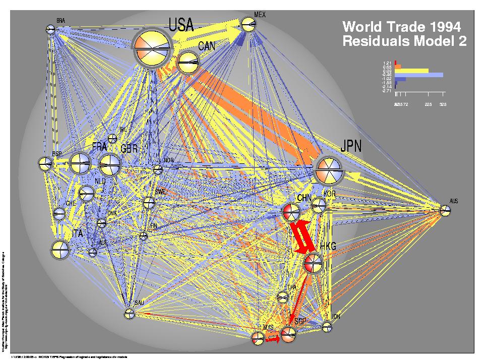
Figure 2: Residuals Model II

Residuals rendered with a color scheme onto the volumes of trade and a simplified world map. The node symbols allow for the reading of the extent to which the national imports (top) and exports (bottom) are misrepresented with a given model.

Use the following links to access two SVG versions of this graphic to explore the image interactively by the accuracy of the flow estimates m2quality.html and by the origin and destination of trade m2country.html .

Including the GDP of all countries to estimate the trade flows dramatically improves the explained variance to 60 percent for the 1994 model and increases the number of (almost) correctly estimated flows from 238 to 325 (as can be read from the distribution in the upper right). While the accuracy of the estimates has improved for many countries, we find that the trade between the US and Japan is still underestimated with this second model. This is also true for much of the trade in the Asian region and for the trade from Asia to the USA. Therefore, the third model includes a dummy for all bilateral trade occurring between countries located on the same ocean: either the Pacific or the Atlantic. This allows for the estimation of the beneficial effect of maritime trade routes and their lower associated transportation costs. For both variables we expect the signs of the coefficients to be positive, indicating that higher trade volumes occur between countries that profit from maritime trade. The inclusion of maritime trade improved the model further to 62.8 percent of explained variance and especially improves the estimates for flows that were miscalculated in model 2. A separate estimate of the two major oceans displays that the parameter estimate for the trade in the Pacific Rim is higher than the estimate for the Atlantic (0.5072 versus 0.3811). Most of the shipping costs seem to be a result of loading and unloading. While the estimate for the trade between Japan and the US is now only moderately misrepresented (too low), the trade between Hong Kong and China, and also somewhat more surprisingly the trade between Korea, Singapore and Malaysia, are consistently estimated too low. We correct further imperfections by including a border dummy for all dyads of countries sharing a common border. The coefficients are expected to be positive. It is more likely that neighboring countries have higher trade volumes. Taking the increased trade volumes between neighboring countries into account, the overall model improves to 64 percent of the explained variance.

While the increase in trade for neighboring countries is found to be quite strong, it is, however, much smaller than the estimate for the impact of the overall distance. Looking at the errors after removing the common border effect from the errors, we still find that the trade in Asia is underestimated to a considerable degree, namely between Hong Kong and China but also the trade between and with Malaysia and Singapore.

Our final approximation also includes dummies for different world regions and allows us to access the degree to which regional trade integration exists in different geographical areas, discounting all explanations that we have introduced through the use of the less complex models. The estimates for the different regions provide information about the extent local economic integration leads to more trade in specific world regions than would be expected from the pure knowledge of distance, size of GDP, maritime and common borders alone. Such an estimate of local integration differs slightly from studies that simply relate to the growth of local trade only. The degree of local integration as it is expected for regional economic areas, the EU, the NAFTA, and the Asian members of APEC respectively denoted by FTA-dummies leads us to expect positive parameter estimates.

log(TRD_ij) = a+DIST_ij^b+GDP_i^c+GDP_j^d+e Border_ij+f Ocean_ij+g FTA_ij+u_ij

We find a further improvement of our model: 69 percent of all variance in world trade is now explained and a correct estimate for more than 339 flows is given.

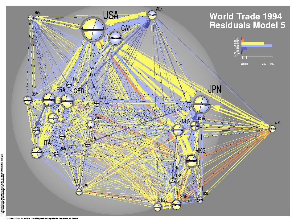
Figure 3: Residuals Model 5

Use the following links to access two SVG versions of this graphic to explore the image interactively by the accuracy of the flow estimates m5quality.html and by the origin and destination of trade m5country.html .

The intraregional trade estimates are strongest for Asia (0.4851), and are insignificant for North America (0.2085) and Europe (-0.1706). Evaluating the error terms of this fifth model, in which now all regional effects are discounted, almost all flows are estimated with modest distortions only. Though this is the most improved model advanced in this article, there still exist some systematic errors as the visualization shows. As the estimate for the trade between Hong Kong and China has improved by treating it as intra-Asian trade, most of the imperfections of the fifth model are still connected to Hong Kong. This effect of Hong Kong's harbor function for mainland China diminished with the Chinese unification. Furthermore, underestimation also occurs for the flows between the countries of the old British Empire, respectively the Commonwealth countries, namely Great Britain, Hong Kong, Singapore and Australia. This leads us to suspect a language effect of international trade: Countries of a single language trade more, an effect that seems to last even in a 'globalized' world economy.

3 The Dynamics of International Economic Integration

In the remainder of this paper we shortly evaluate the dynamics of international economic integration by and large based on the model specifications developed in section 2. We show that the model can contribute to an ongoing debate in International Political Economy. Within this research tradition, the sources of global economic processes are widely discussed. At least three major theories can be distinguished. We refer to these theories as globalization theory, regionalization theory, and macroeconomic imbalances theory. Note, however, that the globalization and regionalization theories lack a coherent microeconomic foundation. Globalization scholars basically accept that globalization is a phenomenon that covers all countries and world regions. In their view, the tendency towards a closer integration stems from a relative easing of international economic transactions compared to national business activity (Frieden & Rogowski, 1996). The costs of international economic exchange relative to within-border transactions exogenously decrease as a result of technological change and political liberalization. Thus, the perspective of a globalizing economy implies that borders and geographical distance get less important: more and more goods are expected to be traded over longer distances due to reduced transportation and transaction costs.

The most widely heeded competitor for the globalization line of reasoning is regionalization theory. Proponents of this theory consider regional dynamics instead of global dynamics as the driving force behind economic internationalization. Regional free trade areas such as NAFTA, the European Union and the ASEAN support this view (Coleman & Underhill 1998). The abolition of tariffs and non-tariff barriers to trade and the establishment of preferential treatments for their member states is aimed to increase the volume of trade within the regions. While the hypothesis of globalization literature implies a general easing of international economic exchange, scholars analyzing regions usually stress the huge and increasing share of interregional trade. In their view, the 'relative easing' of economic transactions not only takes place within the three dominant world regions, namely in Europe (the EU), North America (NAFTA) and Southeast Asia (APEC), but also are caused by regional liberalization measures and are therefore policy-driven.

A third view, shared by just a small fraction of authors, most notably by Paul Krugman (Krugman 1990; Krugman 1996), understands global economic processes as a consequence of global economic imbalances. The increasing budget deficits of the industrialized states and the growing differences in national saving and investment figures serve as an engine of international capital flows: Due to the accounting identities between capital flows and trade in commodities and services these negative capital flows need to be balanced by international trade. Krugman expects bilateral economic interactions to change most between countries with large imbalances of national savings and national investment. International economic integration does not play a mayor role in fueling global economic processes. Countries characterized by a trade deficit are net importers of capital, whereas countries with a savings surplus export capital. The most prominent country with a national saving deficit is the USA; minor capital importers are most of the rapidly developing countries of South-East Asia. Japan on the other hand is the main example of a country with a high surplus.

The three theories differ fundamentally in regard to the expected localization of global economic processes. Globalization theory assumes an overall decrease of transportation costs, which should lead to a diminishing effect of geographical distance in general. There are however no specific expectations how this changes the overall structure of trade. A stronger regionalization on the other hand should increase the estimated parameter of regional estimates due to a relative increase in intra-regional economic transactions and a relative decline in interregional trade. According to the inequality school, we should expect the most change to occur within the Pacific area, while the Transatlantic and European economic relations would remain stable. To our knowledge, none has assumed overlapping processes.

In what follows, we use an extended version of the model developed in section 2 to separate the three dynamics from each other and to estimate their sole contribution to the current dynamics of the world economy. Gravity models are especially useful for these analyses because they allow the separation of the inter-regional from the intra-regional transactions.

Globalization theories deal with spatial consequences of economic processes. While simple gravity models allow for the understanding of the spatial distribution of trade at a given point in time, a model for the dynamics of globalization would be far more complicated. A simple approach, however, is to apply the same models at different points in time and to compare the resulting estimates cross-sectionally. Consistent shifts of certain model components help to identify trends over time and give a rough estimate of their importance. This can be seen as a first attempt to link spatial models to globalization phenomena in the absence of more adequate models.

As yet, economic geography scholars have only modestly engaged in analyzing economic dynamics. To our knowledge, the problem of spatial dynamics has been dealt with in a complex simulation study of Fujita, Krugman and Venables (forthcoming) and just a few spatial models analyze the long run effects of economic differentiation and concentration. Anthony Venables (1995) has assumed that factors of production are less mobile between countries than between different regions of the same country and analyzed the spatial order resulting from this plausible assumption. Krugman and Venables (1995) used this model to show how gradually declining transportation costs lead to a first spontaneous differentiation into a high-wage core and a low-wage periphery and eventually to a convergence of wages as the periphery industrializes. We may conclude that in spite of the considerable fruitfulness of gravity models for the analyses of spatial economic processes, the existing studies do not contribute to the ongoing debate on global economic processes as much as seems to be possible.

We believe that gravity models can contribute to the globalization debate. Globalization theory is still dominated by armchair reasoning while only a handful of scholars engage in sophisticated empirical studies (see for example Garrett 1995, 1998; Hallerberg & Basinger 1998; Lawrence 1996) and a theoretical underpinning of empirical results (Krugman 1995). Economic geography offers the promise to combine the globalization theories with a more rigorous theoretical foundation. Differences between the following model and the model developed before lie essentially on the degree of complexity.

The model estimated below is more complex with regard to the differentiation between world regions and adds additionally the interregional trade between ASIA, North America and Europe. Moreover, the parameters of the model are calculated with data based on 1880 dyads of countries. The data includes the 45⁷ most important trading nations.

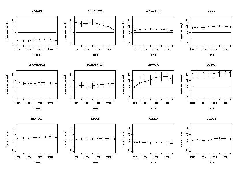
Figure 4: Trends in parameter estimates over time. Cross-sectional estimates for the bilateral trade of 45 countries. Numerical results are given in the table in the appendix.

The parameter estimates for the extended model⁸ are given for eight different points in time in the table in figure 4 respectively. Since we have introduced the basic model components already in section 2, we limit our attention especially to the comparison of the estimates over time.

The decline of the intra-region trade of E.EUROPE and the increase for AFRICA in figure 4 are the strongest changes. These estimates are based on three countries each: CZE, HUN and POL for East Europe, and MAR, TUN and ZAF for AFRICA and show large standard errors.

The other coefficients lead to fairly reasonable and interesting results. Globalization theory nicely explains the decline in the estimated parameter of log(DIST_ij) between 1984 and 1992. However, it is unable to explain why the trade limiting effect of sheer distance declines as rapidly as it does, and is even less well equipped to specify why the negative effect of distance increases between 1992 and 1994. Globalization theorists face a crucial challenge in explaining this aspect. If economic processes were truly global in their character and were the effect of an exogenous easing of international economic transaction, the estimated coefficients of the three dummies for interregional trade, EU/AS, AS/NA, NA/EU should be increasing, thereby indicating that interregional trade is growing (in relative terms), simply because the negative impact of distance on trade diminishes.

Regionalization theory also explains some aspects and ignores others. The rapid increase in the estimated coefficient for intra-North American trade, the growing importance of trade between neighboring countries between 1980 and 1992 supports the regionalization hypothesis. However, the results remain puzzling. The degree of Asian integration sharply declines after 1990, Western European integration peaks in 1986 and most puzzling the estimated coefficient of EUROPE is much smaller than the ASIA coefficient. This seems to indicate that the assumed superiority of European integration is partly misleading, at least if one controls for country size, distance and borders: The estimated coefficient reaches the size of the ASIA coefficient only if we add the border effect to the regional integration effect.

The economic imbalances theory perfectly predicts the sharp increase in the AS/NA coefficient. Trade between Asian and North American countries increases as the American twin deficit worsens. Moreover, since European saving figures are below their Asian counterparts, economic imbalances also nicely predicts that a similar increase does not take place between Europe and North America. To sum up, we gain somewhat mixed results. Each of the three existing theories explains only very small parts of the story of global economic integration. Hence, we should be far from being satisfied with existing reductionistic theories.

4 Conclusion

Multiple Regressions and Network Visualization illustrate that single factor explanations of global economic integration are presumably misleading. On the one hand, we observe that distance still matters: Geography has a huge impact on bilateral trade flows. Even a simple model with three independent variables, namely the gross domestic product of the importer and exporter respectively, as well as the distance between both countries, is a fair approximation to and nicely predicts bilateral trade flows. On the other hand, the strong economic integration between South-East Asia and North America, especially the US, does not entirely follow the pattern of capital exporter/ capital importer as expected by Krugman. In general, however, it seems fair to conclude that the notion of a truly globalized economy is by far less appropriate than the notion of regionalization.

The amount of trade flows differs widely according to the continent the trading partners are located on. Here, the estimated coefficient of the 'Euro-dummy' compared to the coefficients of the North America and Asia-dummies seems to be most puzzling. Given that European countries are close neighbors and institutional barriers to trade have almost completely been removed during the process of European integration, it is hardly trivial to understand why European countries trade less with each other than a dyad located in any other world region. However, even though some results are surprising, we do not believe that they are a methodological artifact. Quite the opposite is the case; gravity models are a good starting point for the empirical analysis of international trade. In the medium run, the newly developing branch of economic geography should improve neoclassical approaches to international trade and bring economic modeling and the raw world of observable facts a bit closer together.

5 Appendix

	1980	1982	1984	1986	1988	1990	1992	1994
Y-Intercept	-13,1164⁴	-12,9857 ⁴	-12,9599 ⁴	-12,8653 ⁴	-12,5309 ⁴	-12,5739 ⁴	-12,3768 ⁴	-12,3748 ⁴
	(0,5049)	(0,4930)	(0,4901)	(0,4345)	(0,4041)	(0,4033)	(0,3843)	(0,3701)
LogDist	-0,7268⁴	-0,7431⁴	-0,7432⁴	-0,6350 ⁴	-0,6260 ⁴	-0,6238 ⁴	-0,6385 ⁴	-0,7083⁴
	(0,0493)	(0,0482)	(0,0488)	(0,0439)	(0,0410)	(0,0406)	(0,0380)	(0,0371)
LogGDPx	1,0090⁴	1,0173 ⁴	0,9797 ⁴	0,9373⁴	0,9291 ⁴	0,9143 ⁴	0,9355 ⁴	0,9402 ⁴
	(0,0291)	(0,0288)	(0,0286)	(0,0248)	(0,0230)	(0,0228)	(0,0218)	(0,0213)
LogGDPm	0,8805 ⁴	0,8604 ⁴	0,8984 ⁴	0,8900 ⁴	0,8594 ⁴	0,8715 ⁴	0,8389⁴	0,8606⁴
	(0,0290)	(0,0287)	(0,0284)	(0,0247)	(0,0229)	(0,0226)	(0,0216)	(0,0211)
EAST-	0,8718 ³	0,7541³	0,7629 ³	0,8715 ⁴	0,7437 ³	0,6019 ³	0,4908 ²	0,2204
EUROPE	(0,2731)	(0,2666)	(0,2698)	(0,2431)	(0,2270)	(0,2247)	(0,2102)	(0,2040)
WEST-	0,1476 ²	0,2464 ⁴	0,2833 ⁴	0,2993 ⁴	0,2638 ⁴	0,2768 ⁴	0,2015 ⁴	0,1640 ⁴
EUROPE	(0,0613)	(0,0596)	(0,0603)	(0,0547)	(0,0514)	(0,0512)	(0,0480)	(0,0463)
ASIA	0,3840 ⁴	0,4555 ⁴	0,4131⁴	0,4884 ⁴	0,5227 ⁴	0,5787⁴	0,5415 ⁴	0,4692⁴
	(0,0586)	(0,0572)	(0,0579)	(0,0521)	(0,0486)	(0,0481)	(0,0451)	(0,0451)
SOUTH-	0,3726 ²	0,2477 *	0,2836 *	0,2138	0,3502 ³	0,3152²	0,2816 ²	0,2719 ²
AMERICA	(0,1509)	(0,1474)	(0,1492)	(0,1344)	(0,1255)	(0,1242)	(0,1161)	(0,1127)
NORTH-	0,0234	0,0952	0,0267	0,0539	0,1334	0,1568	0,2141	0,2664
AMERICA	(0,2726)	(0,2665)	(0,2700	(0,2458	(0,2264)	(0,2241)	(0,2097)	(0,2036)
AFRICA	-0,0638	0,2804	0,4404	0,5488	0,7754 ²	0,8365 ²	0,8593 ²	0,5851 *
	(0,4589)	(0,4483)	(0,4538)	(0,4086)	(0,3814)	(0,3772)	(0,3528)	(0,3426)
OCEAN	1,1533 ²	1,1580³	1,1643 ²	1,1827³	1,1080 ³	1,2284 ³	1,2689 ⁴	1,1916 ⁴
	(0,4573)	(0,4466)	(0,4521)	(0,4071)	(0,3800)	(0,3759)	(0,3516)	(0,3414)
BORDER	0,1619 *	0,1663 *	0,1743 ²	0,2421 ³	0,2596 ⁴	0,2763 ⁴	0,3106⁴	0,2253 ⁴
	(0,0889)	(0,0869)	(0,0880)	(0,0792)	(0,0739)	(0,0731)	(0,0684)	(0,0665)
EU-AS	0,0759²	0,1189 ³	0,1018 ³	0,1038 ³	0,1198⁴	0,1651 ⁴	0,1161 ⁴	0,1111 ⁴
	(0,0372)	(0,0364)	(0,0369)	(0,0333)	(0,0311)	(0,0309)	(0,0289)	(0,0280)
NA-EU	-0,2151 ³	-0,1524 ²	-0,2021 ³	-0,2313 ³	-0,2046 ⁴	-0,2039 ⁴	-0,2529⁴	-0,2940 ⁴
	(0,0690)	(0,0674)	(0,0685)	(0,0613)	(0,0572)	(0,0569)	(0,0533)	(0,0514)
AS-NA	-0,0092	0,0405	-0,0376	0,0046	0,1307 ²	0,1630 ²	0,1264 ²	0,1235 ²
	(0,0780)	(0,0765)	(0,0780)	(0,0696)	(0,0649)	(0,0644)	(0,0604)	(0,0586)

Table 1: Cross-sectional estimates for the bilateral trade of 45 countries

(*) p < 5 % sig ; (2) p < 1% sig; (3) p < 0.1 % sig; (4) p < 0.01 % sig

Standard errors are given in parentheses.

References

: Beck, Nathaniel, and Jonathan Katz, 1995: What to do (and not to do) with Time-Series Cross-Section Data. American Political Science Review 89, pp. 634-647.
: Brandes, Ulrik, 2001: Drawing on Physical Analogies, In: M. Kaufmann and D. Wagner (eds): Drawing Graphs: Methods and Models. Springer LNCS Tutorial 2025: pp. 71-86.
: Brandes, Ulrik (1999): Layout of Graph Visualizations, Dissertation. Universität Konstanz, Fakultät für Mathematik und Informatik.
: Coleman, William D., and Geoffrey Underhill, R.D., 1998: Domestic Politics, Regional Economic Co-operation and Global Economic Integration. Routledge, London.
: Cramer, J., 1986: Econometric Applications of Maximum Likelihood Methods. Cambridge University Press, Cambridge.
: Davidson, Ron, and David Harel, 1996: Drawing Graphs Nicely Using Simulated Annealing. ACM. Transactions on Graphics, vol. 15(4), October 1996, pp. 301-331.
: Eades, Peter, 1984: A heuristic for Graph Drawing. Congressus Numeratum, vol.42, pp. 149-160.
: Freeman, Linton C., 2000: Visualizing Social Networks. Journal of Social Structure, vol. 1(1), February 4, 2000.
: Frieden, Jeffrey, and Ronald Rogowski, 1996: The Impact of the International Economy on National Policies. In: Robert Keohane and Helen Milner: Internationalization and Domestic Policies, Cambridge University Press, Cambridge.
: Fujita, M., P. Krugman, and A. Venables (forthcoming): The Spatial Economy.
: Fruchterman, Thomas, M.J. Edward, and M. Reingold, 1991: Graph Drawing by Force Directed Placement. Software-Practice and Experience vol. 21 (11), pp. 1129-1164.
: Garrett, Geoffrey, 1995: Capital Mobility, Trade, and the Domestic Politics of Economic Policy. International Organization 49, pp. 657-687.
: Garrett, Geoffrey, 1998: Partisan Politics. Cambridge University Press, Cambridge.
: Hagerstrand, T., 1968: A Monte Carlo Approach to Diffusion. In: Statistical Analysis, B.J.L Berry, D.F. Marble (eds). Prentice-Hall, N.J.
: Haggett, P., A. Cliff, and A. Frey, 1977: Locational Analysis in Human Geography. 2nd edition, Edward Arnold, London.
: Hallerberg, Mark, and Scott Basinger, 1998: Internationalization and Changes in Tax Policy in OECD Countries. Comparative Political Studies 31, pp. 321-352.
: Hanushek, Eric, and John E. Jackson, 1977: Statistical Methods for Social Scientists. New York: Academic Press.
: Harris, C. D., 1954: The Market as a Factor in the Localization of Production. Annals of the Association of American Geographers 44, pp. 315-348.
: Haynes, Kingsley E., and A. Stewart Fotheringham, 1984: Gravity and Spatial Interaction Models. Sage: Beverly Hills.
: Kamada, T., and S. Kawai, 1989: An Algorithm for Drawing General Undirected Graphs. Information Processing Letters 31(1), pp. 7-15.
: Johnson, J.C., David Richardson and Jane Richardson 2002: Network Visualization of Social and Ecological Systems. http://iwep.ab.ru/~workshop/johnson/network_visualization.htm
: Kirkby, M.J., P.S. Naden, T.P. Burt, and D.P. Butcher, 1993: Computer Simulation in Physical Geography, Wiley, Chichester, 2nd edition.
: Krempel, Lothar, 2003: Netzwerkvisualisierung: Prinzipien und Elemente einer graphischen Technologie zur multidimensionalen Exploration sozialer Strukturen.
: Krempel, Lothar, 1999: Visualizing Networks with Spring Embedders: Two-mode and Valued Data. American Statistical Association 1999, Proceedings of the Section of Statistical Graphics, Alexandria, VA, pp. 36-45
: Krempel, Lothar and Thomas Plümper, 1999: International Division of Labor and Global Economic Processes: An Analysis of the International Trade in Automobiles. Journal of World-Systems Research, 5, pp. 390-402.
http://csf.colorado.edu/jwsr/archive/vol5/vol5_number3/krempel/index.html
: Krugman, Paul, 1991: Increasing Returns and Economic Geography. Journal of Political Economy 99, pp. 483-499.
: Krugman, Paul, 1992: Geography and Trade. MIT Press, Cambridge.
: Krugman, Paul, 1995: Development, Geography and Economic Theory. MIT Press, Cambridge.
: Krugman, Paul, 1995: Growing World Trade: Causes and Consequences. Brookings Papers on Economic Activity 1, pp. 327-377.
: Krugman, Paul, 1998: Space: The Final Frontier. Journal of Economic Perspectives 12, pp. 161-174.
: Krugman, Paul, and Anthony Venables, 1995: Globalization and the Inequality of Nations. Quarterly Journal of Economics 110, pp. 857-880.
: Lawrence, Robert Z., 1996: Single World, Divided Nations? Brookings Institution, Washington.
: McCallum, John, 1995: National Borders Matter: Canada-US Regional Trade Patterns. The American Economic Review, pp. 615-623.
: Morrill, R., G. L. Gaile, and G. I. Thrall, 1988: Spatial Diffusion. Sage Publications, Newbury Park, USA.
: Obstfeld, Maurice, and Kenneth Rogoff, 1996: Foundations of International Macroeconomics. MIT Press, Cambridge.
: Pred, A.R., 1966: The Spatial Dynamics of Urban Industrial Growth, 1800-1914. MIT Press, Cambridge.
: Thomas, R.W., and R. J. Huggett, 1980: Modeling in Geography A mathematical approach. Harper & Row, London.
: van Beers, Cees, 1998: Labor Standards and Trade Flows of OECD Countries. The World Economy vol. 21(1).
: Venables, Anthony, 1995: Economic Integration and the Location of Firms. American Economic Review Papers and Proceedings 85(2), pp. 296-300.
: White, Halbert, 1980: A Heteroskedasticity-consistent Covariance Matrix and a Direct Test for Heteroskedasticity. Econometrica 48, pp. 817-838.
: Wonnacott, Ronald J. and Thomas H., 1979: Econometrics. John Wiley, New York.

Footnotes:

¹ Max Planck Institute for the Study of Societies, Paul Str.3, D50676 Cologne, Germany. email: krempel@mpi-fg-koeln.mpg.de

² Department of Political Science and Public Administration, University Konstanz, Box D78, D-78457 Konstanz, Germany. email: thomas.pluemper@uni-konstanz.de

³ Because our focus is to obtain cross-sectional estimates for at least two points in time, we had to omit Germany and the former USSR because much of the change in their trade patterns is obviously connected to the political changes in these countries. We also had to exclude Belgium and Taiwan because of missing data. The remaining 26 countries are: AUS, AUT, BRA, CAN, CHE, CHN, DNK, ESP, FIN, FRA, GBR, HKG, IDN, IRE, ITA, JPN, KOR, MEX, MYS, NLD, NOR, SAU, SGP, SWE, THA, USA

⁴ We implicitly assume that bilateral trade between one dyad does not affect the bilateral trade between another dyad of countries. Even through this is almost certainly a false assumption, there is no evidence that any other simple assumption is more appropriate.

⁵ How to represent geographic space is a problem which has a very long history. While 2-dimensional maps have been used for several thousand years, the oldest globes known today date back to the 16th century. How to best map locations from the globe to two-dimensional space has been a core problem of cartography for several centuries. Today geography uses more than 20 different projection rules.

All metric embeddings share the problem that the maximum size that can be used to display trade volumes is very limited. As trade volumes are considerably related to distance, trade between neighboring countries is higher than volumes between distant countries and therefore difficult to display.

The representation of geographic distances with statistical tools or automatic drawing routines leads to a couple of interesting alternatives and questions. Since the country capitals are locations on the surface of a sphere, we could use their 3-dimensional coordinates and feed them directly to 3D visualization tools like Mage (Freeman 2000, Johnson, Jeffery C, David Richardson and Jane Richardson 2002). Mage allows for the exploration of such a mapping sequentially, by taking different viewpoints. The interactive inspection of the trade flows around the globe and their attributes however requires intensive navigation.

An advantage of two-dimensional maps is that they can give a complete view of a sphere's surface. Cartographic maps are more or less distorted metric representations of the geographic distances and have the same limitations as other metric approaches to display the complete trade information in a single image. Thematic atlases which display trade flows typically show only some of the most important shipping destinations.

Another interesting option is to apply multivariate statistical procedures to the matrix of geographic distances, for instance to reconstruct a spherical or 2-dimensional representation of the distance data: what kind of globe or map can be reconstructed with the help of statistical procedures from the geographic distances is a first question; a second whether such maps are well suited to communicate the trade information.

⁶ Mainstream economics almost completely ignored spatial issues and therefore also neglected geographic aspects the gravity models are devoted to. It is fair to say that work on economic location lied outside the intellectual core of economics. This neglect had a simple reason: Almost all neoclassical authors assume perfect markets. Hence, to say anything useful and interesting about geographic aspects of economic exchange, it is necessary to relax the assumptions of constant returns and perfect competition that dominates economic textbooks and journals. For decades, economists have been unwilling to do so. This picture has changed dramatically only during the last decade. Gravity models have become fairly popular in economics, mainly because economists have turned their attention to the location of economic activity (Krugman 1998: 161). Paul Krugman (1991; 1992; 1998), Alan Deardorff (1997) and Anthony Venables (1995) among others have begun to integrate economic geography into economics.

⁷ This adds 19 additional countries to those of model one: ARG, BEL, CHL, COL, CZE,
GRC, HUN, IND, ISR, MAR, NZL, PAK, PHL, POL, PRT, TUN, TUR, VEN, ZAF

⁸ The difference between the 1880 actually included cases and the 1980 possible dyads results from the exclusion of dyads, in which of the total amount of trade actually reported by one country does not exceed $10,000 per year. This omission can be justified by the fact that the data become fairly imprecise and extremely volatile when the trade of two countries is very small.

File translated from T_EX by T_TH, version 2.51.
On 23 Dec 2002, 17:03.