Relations, Species, and Network Structure*
John Skvoretz
Department of Sociology, University of South Carolina
Katherine Faust
Department of Sociology, University of California, Irvine
* For their encouragement and suggestions on the research, we thank H. Russell Bernard, Linton Freeman, and A. Kimball Romney.Ā Discussion with Tom Snijders on the p* models was most helpful.Ā We also thank Mike Burton for suggesting the matrix permutation approach.Ā On a more personal note, we would like to acknowledge and celebrate the influence of Linton Freeman on our careers.Ā On a visit to Lehigh University in the Fall of 1968 to give a talk, Lin advised John, a double major in Sociology and Mathematics, to do his graduate work at Pittsburgh with a young professor named Tom Fararo, thereby setting in motion a life-long interest in networks and structure.Ā And, it was after Lin joined the School of Social Sciences at the University of California, Irvine in 1979 as dean and catalyst for the Social Networks Program that Katie's research interests turned to social networks.Ā It was also Lin who encouraged Katie to go to the University of South Carolina, thereby making possible the collaboration that led to this research.
ABSTRACT: The research we report here tests the "Freeman-Linton Hypothesis" which we take as arguing that the structure of a set of relational ties over a population is more strongly determined by type of relation than it is by the type of species from which the population is drawn.Ā Testing this hypothesis requires characterizing networks in terms of the structural properties they exhibit and comparing networks based on these properties.Ā We introduce the idea of a structural signature to refer to the profile of effects of a set of structural properties used to characterize a network.Ā We use methodology described in Faust and Skvoretz (forthcoming) for comparing networks from diverse settings, including different animal species, relational contents, and sizes of the communities involved.Ā Our empirical base consists of 80 networks from three kinds of species (humans, non-human primates, non-primate mammals) and covering distinct types of relations such as influence, grooming, and agonistic encounters.Ā The methods we use allow us to scale networks according to the degree of similarity in their structuring and then to identify sources of their similarities.Ā Our work counts as a replication of a previous study that outlined the general methodology.Ā However, as compared to the previous study, the current one finds less support for the Freeman-Linton Hypothesis.
| "My overall goal... is to learn something basic about the foundations and consequences of the sociability of social animals." |
| Linton Freeman, 1999, Research
in Social Networks (http://eclectic.ss.uci.edu/~lin/work.html) |
| Ā |
| "... just as the physical differences between men and apes diminish in importance and cease to be a bar to a relationship when they are studied against the background of mammalian variation, the differences in behavior diminish in importance when they are seen in their proper perspective."Ā |
| "... human and animal behavior can be shown to have so much in common that the gap ceases to be of great importance." |
| ĀĀRalph Linton, 1936, The Study of Man (New York:Ā The Free Press) |
Ā
Introduction
The passages of Ralph Linton quoted above suggest that the behavioral commonalities between humans and animals are substantial.Ā The claim would extend to social behavior, in particular, behavior in regard to others of the same species, "the sociability of the social animals."Ā This view is echoed in Lin Freeman's work.Ā That is, both authors would contend that the networks of baboons and school children, of cattle and bank clerks, and of fraternity brothers and ponies would be similarly structured whenever the nature of the behavior defining the connections was common to both networks.Ā In this paper we explore what we will call the Freeman-Linton Hypothesis, named after the scholars quoted above.Ā In particular, we examine 80 different networks from three types of species (humans, non-human primates, and non-primate mammals), varying in size from 4 to 73 units.Ā Many distinct types of relations are included:Ā from liking, influence and grooming to disliking and victory in agonistic encounters.Ā Our specific research question is whether patterning in a network can be better predicted by type of animal or type of relation.Ā The Freeman-Linton hypothesis leads us to expect that type of relation will matter much more than type of social animal.
To investigate this hypothesis requires a methodology that allows the comparison of many networks even though they may vary dramatically in size, in type of social animal, and in relational contents.Ā The methodology should provide an abstract way of characterizing the structure of a network apart from the particular individuals involved.Ā It should also provide a set of guiding principles for what it means to say that two networks are similarly structured.Ā The method we build on has been described in detail elsewhere (Faust and Skvoretz forthcoming).Ā In the next section we outline the steps in that method.Ā We then apply it to our networks, replicating the original analysis, which was restricted to a smaller set of networks (42 in number).Ā We also extend the original analysis to consider systematically sources of variation in network structuring among networks of different species and different types of relations.Ā We conclude the paper with a discussion of directions for future work with particular attention to the theoretical questions our project may address.
Ā
Representation of the Structural Signature of a Network
Faust and Skvoretz (forthcoming) propose a method that allows researchers to
measure the similarity between pair of networks and to look at the overall patterning
of similarities among a large collection of networks from diverse settings.Ā
Their basic argument is that two networks are similarly structured, that is,
have the same structural "signature," to the extent that the networks
exhibit the same structural properties and to the same degree.Ā One way
to quantify the magnitudes and directions of network's structural properties
is to use a statistical model.Ā In that case, two networks are similarly
structured if the probability of a tie between i and j is affected by the same
set of structural factors to the same degree in both networks.Ā To explicate
this idea, consider a single structural factor, say, mutuality and two networks:Ā
A is a network of advice ties between sales personnel and B is a network of
helping relations between blue-collar workers.Ā Mutuality, the tendency
for actor i to return a tie to actor j if j sends a tie to i, might be one structural
factor that affects the probability of a tie between two actors in either network
A or network B.Ā Tendencies toward mutuality have long been a concern of
social network analysts (Katz and Powell 1955; Katz and Wilson 1956) and the
measurement of mutuality remains a focus of contemporary research (Mandel 2000).Ā
It is a "structural" factor because it refers to a property of the
arrangement of ties in any pair in the graph rather than to properties of the
individuals composing the pair.
With just this one factor, Faust and Skvoretz would propose that networks A
and B are similarly structured if a tendency toward mutuality is present or
absent in both networks and to the same degree.Ā Specifically, their method
calibrates the strength of such structural tendencies in terms of measures of
impact that are invariant across networks that differ in size and overall density.Ā
Therefore, strictly speaking, networks A and B are similarly structured if the
standardized tendency toward mutuality is identical in both networks.Ā
Of course, with just one structural factor, fine discriminations among the structural
patterns in different networks are just not possible.Ā Networks that may
be structurally distinct for other reasons (such as different tendencies towards
transitivity) would be classed as similar because only one structural factor,
mutuality, has been taken into account.
As additional factors are considered, finer and finer discriminations among
entire sets of networks become possible.Ā But these finer distinctions
require measuring multiple structural properties of the networks.Ā One
could amass a collection of graph-based indices calculated on each network (mutuality,
transitivity, ...) and then compare these collections, but a more coherent approach
is to estimate a set of effects simultaneously in the context of a statistical
model for the network.Ā Thus the first step in the comparison methodology
proposed by Faust and Skvoretz (forthcoming) is to estimate statistical models
for the probability of a graph in which the set of predictor variables is expanded
beyond simple mutuality.Ā Until recently, no statistical models were able
to incorporate any structural effects beyond mutuality.Ā However, with
the development of family of models known as p* such investigations became possible
(Anderson et al. 1999;Ā Crouch et al. 1998; Pattison and Wasserman 1999;
Wasserman and Pattison 1996; Robins, Pattison, and Wasserman 1999).Ā Faust
and Skvoretz use a p* model that includes six structural properties:Ā mutuality,
transitivity, cyclical triples, and star configurations (in-stars, out-stars,
and mixed stars) as illustrated in Figure 1.Ā The model is based on what
Frank and Strauss (1986) call a "Markov" graph assumption.Ā This
assumption stipulates that the state of a tie between i and j can only be influenced
by the state of a tie between two other actors if at least one of these other
actors is i or j.Ā Put another way, there is no impact "at a distance,"
meaning that the state of the tie between x and y cannot impact the state of
the tie between w and z if x and y are complete different persons than w and
z.Ā Furthermore, the model assumes that the Markov graph effects are homogeneous,
that is, unrelated to specific labeled identities of actors.Ā Thus these
effects are "purely structural" in that they do not depend the labels
attached to the nodes.
 Ā a.Ā Mutual |
 Ā b. Out 2-star |
 Ā c.Ā In 2-star |
Ā d.Ā Mixed 2-star |
 Ā e.Ā Transitive triple |
 Ā f.Ā Cyclic triple |
Ā
A p* model expresses the probability of a digraph G as a
log-linear function of a vector of parameters ![]() , an
associated vector of digraph statistics x(G),
and a normalizing constant Z(
, an
associated vector of digraph statistics x(G),
and a normalizing constant Z(![]() ):
):
| (1)Ā |
The normalizing constant insures that the probabilities sum to
unity over all digraphs.Ā The ![]() parameters express how
various "explanatory" properties of the digraph affect
the probability of its occurrence.Ā The explanatory
properties of the graph include the structural factors, like
mutuality and transitivity mentioned above.Ā The model we
use stipulates that the probability of a graph is a log-linear
function of the number of mutual dyads, the number of out
2-stars, the number of in 2-stars, the number of mixed 2-stars,
the number of transitive triples, and the number of cyclical
triples.Ā If the resulting parameter estimate for a specific
property is large and positive, then graphs with that property
have large probabilities.Ā For example, if mutuality has a
positive coefficient, then a graph with many mutual dyads has a
higher probability than a graph with few mutual dyads.Ā Or,
if the cyclical triple property has a negative coefficient, then
a graph with many cyclical triples has a lower probability than a
graph with few cyclical triples.Ā Thus, the resulting
parameter estimates associated with the structural properties
capture the importance of these properties for characterizing the
network under study.Ā The set of
parameters express how
various "explanatory" properties of the digraph affect
the probability of its occurrence.Ā The explanatory
properties of the graph include the structural factors, like
mutuality and transitivity mentioned above.Ā The model we
use stipulates that the probability of a graph is a log-linear
function of the number of mutual dyads, the number of out
2-stars, the number of in 2-stars, the number of mixed 2-stars,
the number of transitive triples, and the number of cyclical
triples.Ā If the resulting parameter estimate for a specific
property is large and positive, then graphs with that property
have large probabilities.Ā For example, if mutuality has a
positive coefficient, then a graph with many mutual dyads has a
higher probability than a graph with few mutual dyads.Ā Or,
if the cyclical triple property has a negative coefficient, then
a graph with many cyclical triples has a lower probability than a
graph with few cyclical triples.Ā Thus, the resulting
parameter estimates associated with the structural properties
capture the importance of these properties for characterizing the
network under study.Ā The set of ![]() parameters
forms the structural signature of the network.[1]
parameters
forms the structural signature of the network.[1]
The equation (1) form of the model cannot be directly estimated.Ā Rather
the literature proposes an indirect estimation procedure in which focuses on
the conditional logit, the log of the probability that a tie exists between
i and j divided by the probability it does not, given the rest of the graph
(Strauss and Ikeda 1990; Wasserman and Pattison 1996).Ā Derivation of this
conditional logit shows it to be an indirect function of the explanatory properties
of the graph.Ā Specifically, it is a function of the difference in the
values of these variables when the tie between i and j is present versus when
it is absent, as specified in the following equation:
(2)Ā ![]()
where G-ijĀ is the digraph including all adjacencies except
the i,jth one, G+ is G-ij with xij=1
while G- is G-ij with xij=0.Ā In the logit
form of the model, the parameter estimates have slightly different interpretations.Ā
For instance, if the cyclical triple property has a negative coefficient, then
in the equation (1) version, we may say that a graph with many cyclical triples
has a lower probability than a graph with few cyclical triples.Ā In the
equation (2) version, the interpretation is that the log odds on the presence
of a tie between i and j declines with an increase in the number of cyclical
triples that would be created by its presence.Ā (Technically, however,
interpretation is best phrased in terms of the probability of the graph.)Ā
The importance of the logit version of the model lies in the fact that, as Strauss
and Ikeda (1990) show, the logit version can be estimated, albeit approximately,
using logistic regression routines in standard statistical packages.[2]Ā
The significance for our problem of identifying the structural signature of
a network is that it is possible to build and estimate models that capture multiple
structural effects.Ā We are no longer limited to a structural signature
built on only one or two factors.Ā In the research we report in the next
section each network has a six-dimensional signature defined by the parameter
estimates for the effects of the six structural factors diagrammed in Figure
1.Ā We also present several ways to compare the signatures of different
networks, looking for similarities and differences.Ā One of these ways
extends the work of Faust and Skvoretz (forthcoming) who use parameter estimates
from different networks to generate sets of predicted tie probabilities for
focal networks and then compare the sets of predicted probabilities using an
Euclidean distance function.Ā Another way, new to the present research,
explores the structural signatures based directly on the parameter estimates.
In all comparisons, we seek to assess the tenability of the Freeman-Linton hypothesis.Ā
Specifically, we want to compare the structural signatures of human networks
to the structural signatures of the networks of other species.Ā If we find,
in fact, that the signatures differ, we want to see how much of the difference
can be accounted for by "controlling for" relational type.Ā That
is, the Freeman-Linton hypothesis would predict that any difference in the aggregate
between human networks and the networks of other species would disappear once
we take into account relational type.Ā In other words, the hypothesis holds
that the nature of the behavior defining the connections, not species of social
animal, is the fundamental factor determining a network's properties and thus
its structural signature.Ā These are the implications of the hypothesis
we seek to evaluate.
Ā
Comparisons of Structural Signatures
Table 1 lists the 80 networks we use to evaluate the Freeman-Linton hypothesis and to illustrate our methodology of comparison.Ā The networks range in size from four colobus monkeys to 73 high school boys.Ā The ties composing the networks also vary from advice relations and friendship ties to victories in agonistic encounters.Ā Each of the networks that we compare is represented by a 0,1 adjacency matrix (created by dichotomizing all non-zero entries equal 1 if the original relation was valued).Ā More details about each of the networks can be found in the Appendix.
Table 1.Ā Description of Networks
| Label | Description | N |
Type of Animal |
Positive or Negative Relation |
Observed or Reported Relation |
| baboonf | dominance between baboons (Hall and DeVore) | 10 |
primate |
negative |
observed |
| baboonm1 | dominance between male baboons (Hall and DeVore) | 6 |
primate |
negative |
observed |
| baboonm2 | dominance between male baboons (Hall and DeVore) | 6 |
primate |
negative |
observed |
| baboonm3 | outcomes of agonistic bouts between male baboons (Hausfater) | 21 |
primate |
negative |
observed |
| banka | advice in a bank office (Pattison et al.) | 11 |
human |
positive |
reported |
| bankc | confiding in a bank office (Pattison et al.) | 11 |
human |
positive |
reported |
| bankf | close friends in a bank office (Pattison et al.) | 11 |
human |
positive |
reported |
| banks | satisfying interaction in a bank office (Pattison et al.) | 11 |
human |
positive |
reported |
| bkfrac | rating of interaction frequency in a fraternity (Bernard et al.) | 58 |
human |
positive |
reported |
| bkhamc | rating of interaction frequency between ham radio operators (Bernard et al.) | 44 |
human |
positive |
reported |
| bkoffc | top rank order of interaction frequency in an office (Bernard et al.) | 40 |
human |
positive |
reported |
| bktecc | top rank order of interaction frequency in a technical group (Bernard et al.) | 34 |
human |
positive |
reported |
| camp92 | top rank order of interaction frequency in "Camp" (Borgatti et al.) | 18 |
human |
positive |
reported |
| cattle | contests between dairy cattle (Schein and Fohrman) | 28 |
mammal |
negative |
observed |
| cole1 | friendship at time 1 between adolescents (Coleman) | 73 |
human |
positive |
reported |
| cole2 | friendship at time 2 between adolescents (Coleman) | 73 |
human |
positive |
reported |
| colobus1 | non-agonistic social acts between colobus monkeys (Dunbar and Dunbar) | 4 |
human |
positive |
observed |
| colobus2 | non-agonistic social acts between colobus monkeys (Dunbar and Dunbar) | 5 |
human |
positive |
observed |
| colobus3 | non-agonistic social acts between colobus monkeys (Dunbar and Dunbar) | 9 |
human |
positive |
observed |
| eiesk1 | EIES data, rating of acquaintanceship (Freeman and Freeman) | 32 |
human |
positive |
reported |
| eiesk2 | EIES data, rating of acquaintanceship (Freeman and Freeman) | 32 |
human |
positive |
reported |
| eiesm | EIES data (Freeman and Freeman) | 32 |
human |
positive |
observed |
| fifth | friendships between fifth graders (Anderson et al.) | 22 |
human |
positive |
reported |
| fourth | friendships between fourth graders (Anderson et al.) | 24 |
human |
positive |
reported |
| ka | advice between managers (Krackhardt) | 21 |
human |
positive |
reported |
| kapfti1 | instrumental work relations in a tailor shop, time 1 (Kapferer) | 39 |
human |
positive |
reported |
| kapfti2 | instrumental work relations in a tailor shop, time 2 (Kapferer) | 39 |
human |
positive |
reported |
| kf | Krackhardt, friendship between managers | 21 |
human |
positive |
reported |
| kids1 | initiated agonism between children (Strayer and Strayer) | 17 |
human |
negative |
observed |
| kids2 | dominance among nursery school boys (McGrew) | 19 |
human |
negative |
observed |
| medical | physicians (Coleman, Katz and Menzel) | 32 |
human |
positive |
reported |
| newc0 | top rankings of friendship in a fraternity, week 0 (Newcomb) | 17 |
human |
positive |
reported |
| newc0n | bottom rankings of friendship in a fraternity, week 0 (Newcomb) | 17 |
human |
negative |
reported |
| newc1 | top ranking of friendship in a fraternity, week 1 (Newcomb) | 17 |
human |
positive |
reported |
| newc1n | bottom rankings of friendship in a fraternity, week 1 (Newcomb) | 17 |
human |
negative |
reported |
| newc10 | top ranking of friendship in a fraternity, week 10 (Newcomb) | 17 |
human |
positive |
reported |
| newc10n | bottom rankings of friendship in a fraternity, week 10 (Newcomb) | 17 |
human |
negative |
reported |
| newc11 | top ranking of friendship in a fraternity, week 11 (Newcomb) | 17 |
human |
positive |
reported |
| newc11n | bottom rankings of friendship in a fraternity, week 11 (Newcomb) | 17 |
human |
negative |
reported |
| newc12 | top ranking of friendship in a fraternity, week 12 (Newcomb) | 17 |
human |
positive |
reported |
| newc12n | bottom rankings of friendship in a fraternity, week 12 (Newcomb) | 17 |
human |
negative |
reported |
| newc13 | top ranking of friendship in a fraternity, week 13 (Newcomb) | 17 |
human |
positive |
reported |
| newc13n | bottom rankings of friendship in a fraternity, week 13 (Newcomb) | 17 |
human |
negative |
reported |
| newc14 | top ranking of friendship in a fraternity, week 14 (Newcomb) | 17 |
human |
positive |
reported |
| newc14n | bottom rankings of friendship in a fraternity, week 14 (Newcomb) | 17 |
human |
negative |
reported |
| newc15 | top ranking of friendship in a fraternity, week 15 (Newcomb) | 17 |
human |
positive |
reported |
| newc15n | bottom rankings of friendship in a fraternity, week 15 (Newcomb) | 17 |
human |
negative |
reported |
| newc2 | top ranking of friendship in a fraternity, week 2 (Newcomb) | 17 |
human |
positive |
reported |
| newc2n | bottom rankings of friendship in a fraternity, week 2 (Newcomb) | 17 |
human |
negative |
reported |
| newc3 | top ranking of friendship in a fraternity, week 3 (Newcomb) | 17 |
human |
positive |
reported |
| newc3n | bottom rankings of friendship in a fraternity, week 3 (Newcomb) | 17 |
human |
negative |
reported |
| newc4 | top ranking of friendship in a fraternity, week 4 (Newcomb) | 17 |
human |
positive |
reported |
| newc4n | bottom rankings of friendship in a fraternity, week 4 (Newcomb) | 17 |
human |
negative |
reported |
| newc5 | top ranking of friendship in a fraternity, week 5 (Newcomb) | 17 |
human |
positive |
reported |
| newc5n | bottom rankings of friendship in a fraternity, week 5 (Newcomb) | 17 |
human |
negative |
reported |
| newc6 | top ranking of friendship in a fraternity, week 6 (Newcomb) | 17 |
human |
positive |
reported |
| newc6n | bottom rankings of friendship in a fraternity, week 6 (Newcomb) | 17 |
human |
negative |
reported |
| newc7 | top ranking of friendship in a fraternity, week 7 (Newcomb) | 17 |
human |
positive |
reported |
| newc7n | bottom rankings of friendship in a fraternity, week 7 (Newcomb) | 17 |
human |
negative |
reported |
| newc8 | top ranking of friendship in a fraternity, week 8 (Newcomb) | 17 |
human |
positive |
reported |
| newc8n | bottom rankings of friendship in a fraternity, week 8 (Newcomb) | 17 |
human |
negative |
reported |
| nfponies | threats between ponies (Tyler) | 13 |
mammal |
negative |
observed |
| prison | friendship in a prison (MacRae) | 67 |
human |
positive |
reported |
| rhesus1 | fights between adult female rhesus monkeys (Sade) | 7 |
primate |
negative |
observed |
| rhesus2 | fights between yearling rhesus monkeys (Sade) | 5 |
primate |
negative |
observed |
| rhesus4 | fights between adult rhesus monkeys (Sade) | 10 |
primate |
negative |
observed |
| rhesus5 | fights between adult rhesus monkeys (Sade) | 12 |
primate |
negative |
observed |
| rhesus6 | fights between adult rhesus monkeys (Sade) | 10 |
primate |
negative |
observed |
| sampdes | disesteem between monks (Sampson) | 18 |
human |
negative |
reported |
| sampdlk | dislike between monks (Sampson) | 18 |
human |
negative |
reported |
| sampes | esteem between monks (Sampson) | 18 |
human |
positive |
reported |
| sampin | influence between monks (Sampson) | 18 |
human |
positive |
reported |
| samplk | liking between monks (Sampson) | 18 |
human |
positive |
reported |
| sampnin | negative influence between monks (Sampson) | 18 |
human |
negative |
reported |
| sampnpr | negative praise (blame) between monks (Sampson) | 18 |
human |
negative |
reported |
| samppr | praise between monks (Sampson) | 18 |
human |
positive |
reported |
| third | friendship between third graders (Anderson et al.) | 22 |
human |
positive |
reported |
| vcbf | best friends between seventh graders (Robins et al.)Ā | 29 |
human |
positive |
reported |
| vcg | get on with between seventh graders (Wasserman and Pattison 1996)Ā | 29 |
human |
positive |
reported |
| vcw | work with between seventh gradersĀ (Wasserman and Pattison 1996)Ā | 29 |
human |
positive |
reported |
First, for each data set, we estimate the standardized
coefficients for a p* model that expresses the conditional
probability of a tie as a function of six structural factors:
mutuality, out 2-stars, in 2-stars, mixed 2-stars, transitive
triples, and cyclical triples.Ā Second, we use these
standardized parameter estimates and the standardized change
scores in these structural factors to calculate the predicted
probability of a tie in each i,j pair in each data set using as
coefficients the parameter estimates from its own model and from
each of the remaining 79 models.Ā Thus for each data set, we
have 80 sets of predicted probabilities, one from each set of
parameter estimates including the set of estimates from the focal
data set itself.Ā The third step uses the Euclidean distance
function:
(3)Ā 
where d(t,y) is the distance between a target network t and a
predictor network y, pt(i,j) is the probability of the
tie between i and j in network t calculated from its own p*
estimates, py(i,j) is the probability of the tie
between i and j in network t predicted by the p* parameter
estimates from network y, and gt is the size of
network t.Ā The distance is a (dis)similarity score between
the predicted probabilities from the estimates derived from t,
the target network itself, and the predicted probabilities from
the estimates derived from y, one of the other 79 networks.
The 80 by 80 matrix of dissimilarity scores is the input data for
two of our three comparisons of network structural
signatures.Ā The first operation follows the methodology of
Faust and Skvoretz (forthcoming) and uses correspondence analysis
to represent the proximities among all of the networks.Ā The
resulting configuration is interpreted in light of the type of
social animal and the type of relation.Ā The second
operation uses matrix permutation tests to model the
dissimilarity scores as linear functions of predictor variables
including type of social animal and type of relation.Ā The
third comparison of the structural signatures of the 80 networks
directly inspects the standardized parameter estimates
themselves, comparing their mean values across categories of
animal type and relation type.
Correspondence analysis results.Ā Correspondence analysis involves a singular value decomposition of an appropriately scaled matrix.Ā Entries in the input matrix are divided by the square root of the product of the row and column marginal totals, prior to singular value decomposition.Ā Correspondence analysis is used because it does not require symmetric input data.Ā Since correspondence analysis requires that data refer to similarities rather than dissimilarities, we rescale the Euclidean distances by subtracting each from a large positive constant prior to doing the correspondence analysis (Carroll, Kumbasar, and Romney 1997).Ā The matrix of similarities we analyze is not symmetric, that is, the distance between network x's prediction for network y and network y's prediction for its own data does not, in general, equal the distance between y's prediction for network x and network x's prediction for its own data.Ā In the following graphs we present the column scores from correspondence analysis of the matrix of similarities among the networks.Ā Column scores show similarities among networks in terms of the predictions they make for other networks.Ā Thus in the figures two networks are close together if they similarly predict other networks in the collection.
The following graphs show the results of the correspondence analysis in the aggregate and then disaggregated by species and type of relation.Ā Species is a categorical variable taking on three values, humans, non-human primates and non-primate mammals.Ā We highlight the contrast between humans and non-human primates because we have relatively few (only 2) networks among mammals in our set of 80 cases.Ā Relations are first categorized by how they were collected:Ā observation or reported by respondent.Ā Obviously this is confounded with the type of animal since only humans provided reports of their ties to others.Ā Second, we categorize the relation as either positive or negative.Ā Grooming, advice seeking, liking, etc. are considered positive, whereas dominance, agonistic encounters, and disliking are negative.Ā This leads to four types: observed positive, observed negative, reported positive, or reported negative.
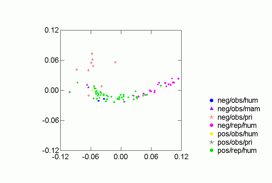
Figures 2-6 display results of the correspondence analysis. Figure 2 shows the location of each data set in the first two dimensions. The closer together two networks are the more similar are their predictions for the other networks in the collection. Thus, for example, "baboonnm2" is relatively far from "kids1" and so the two networks make very different predictions for other networks. Figures 3 through 6 analyze the location of the networks based on type of animal and type of relation. We present 68.2% confidence ellipses around the networks, centered on a category’s means along the first two dimensions with orientation determined by the covariance of the scores of the category’s networks on the two dimensions. Larger ellipses mean more variability in the location of networks of a certain type in the two dimensional space. For mutually exclusive categories like, say, humans and non-human primates, the smaller the overlap of the respective ellipses, the more distinctive is the region in two dimensional space occupied by networks in one category as opposed to the other.
Figures 2-6 display results of the correspondence analysis.Ā Figure 2a shows the location of each network in the first two dimensions.Ā The color and shape of the points code whether the valence of the relation is "positive" or "negative" (as defined below), whether it was recorded by observers or reported by network participants, and the kind of animal involved (human or non-human primate).Ā Figure 2b is another version of the same figure, but with each point labeled by the network it represents.Ā These labels and descriptions of the networks are in Table 1. In both figures 2a and 2b the closer together two networks are the more similar are their predictions for the other networks in the collection.Ā Thus, for example, "baboonnm2" is relatively far from "kids1" and so the two networks make very different predictions for other networks.Ā Figures 3 through 6 analyze the location of the networks based on type of animal and type of relation.Ā We present 68.2% confidence ellipses around the networks, centered on a category's means along the first two dimensions with orientation determined by the covariance of the scores of the category's networks on the two dimensions.Ā Larger ellipses mean more variability in the location of networks of a certain type in the two dimensional space.Ā For mutually exclusive categories like, say, humans and non-human primates, the smaller the overlap of the respective ellipses, the more distinctive is the region in two dimensional space occupied by networks in one category as opposed to the other.
Figure 2. Correspondence Analysis of Similarities between Networks, Column Scores
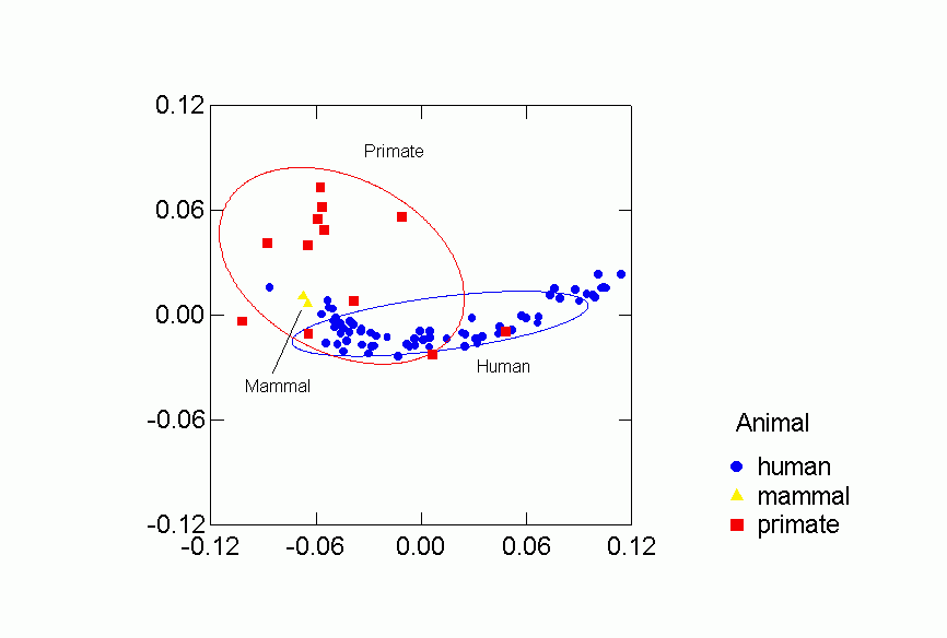
Figure 3. Confidence Ellipses for Type of Animal Overlaid
on Correspondence Analysis
of Similarities between Networks, Column Scores
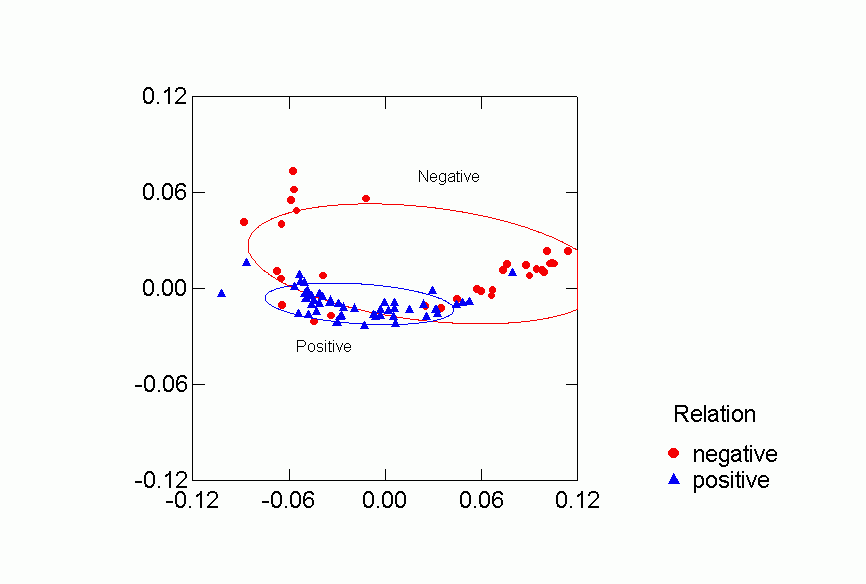
Figure 4. Confidence Ellipses for Positive or Negative Relation
Overlaid on Correspondence Analysis of Similarities between Networks, Column
Scores
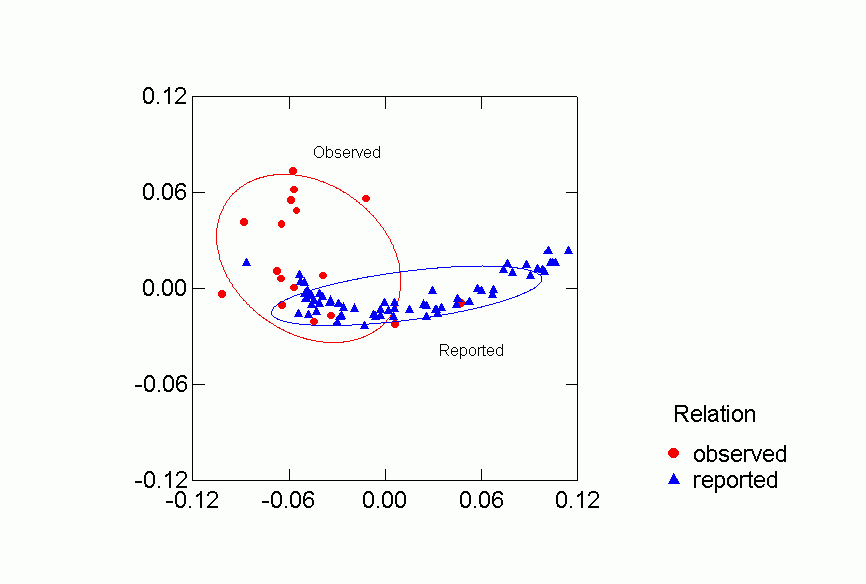
Figure 5. Confidence Ellipses for Observed or Reported Relation
Overlaid on Correspondence Analysis of Similarities between Networks, Column
Scores
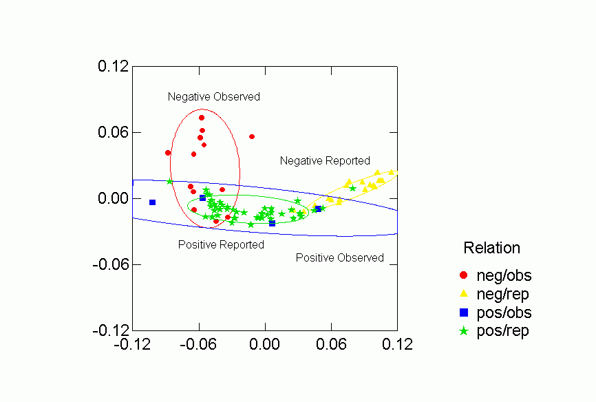
Figure 6. Confidence Ellipses for Type of Relation (Observed
or Reported, Positive or Negative) Overlaid on Correspondence Analysis of Similarities
between Networks, Column Scores
Each of the classifications contributes to understanding the clustering of
the networks in the two dimensional space.Ā Despite some overlap, human
and primate networks are found in different regions, and so too are positive
vs. negative and observed versus reported networks.Ā Positive reported
networks are clearly distinguished from negative reported networks - their confidence
ellipses do not overlap at all.Ā Positive observed and negative observed
overlap and both are more variable than either of the reported relations.Ā
Problematic for the Freeman-Linton hypothesis is the clear distinction between
the networks of different species particularly humans vs. nonhuman primates.Ā
The data remain problematic for this hypothesis in an analysis of variance comparing
column scores along the first three dimensions between categories of the classificatory
variables, as reported in Table 2.Ā Table 2 uses the proportion reduction
in error (PRE) in dimension scores due to the categorical grouping variables,
as measured by the correlation ratio squared, ![]() .Ā
Type of animal is an important distinction along the first and second dimensions
of the correspondence analysis.Ā The kind of relation, especially the four
types differentiating observed vs. reported and positive vs. negative simultaneously,
is an important aspect of all three dimensions.Ā But it is difficult to
maintain the position that type of relation is more important than type of animal
in distinguishing among the networks.Ā To investigate this issue, we return
to the distances between the networks and examine them directly to answer the
question:Ā if we control for relation type, does the effect of animal type
disappear?
.Ā
Type of animal is an important distinction along the first and second dimensions
of the correspondence analysis.Ā The kind of relation, especially the four
types differentiating observed vs. reported and positive vs. negative simultaneously,
is an important aspect of all three dimensions.Ā But it is difficult to
maintain the position that type of relation is more important than type of animal
in distinguishing among the networks.Ā To investigate this issue, we return
to the distances between the networks and examine them directly to answer the
question:Ā if we control for relation type, does the effect of animal type
disappear?
| Ā | Type of Animal1 |
Observed or |
Positive or |
Type of Relation2 |
| Dimension | Ā | Ā | Ā | Ā |
| 1 | 0.16** |
0.20** |
0.13** |
0.67** |
| 2 | 0.34** |
0.22** |
0.36** |
0.46** |
| 3 | 0.04 |
0.01 |
0.02 |
0.17* |
* p < .05 1 ĀType of
animal: human, non-human primate, non-primate mammal |
||||
Matrix permutation test results.Ā A matrix permutation
test allows us to test directly whether distances between
networks are significantly smaller when they are measured on the
same kind of animal than when they are measured on different
kinds of animals, whether they are smaller when both networks
express the same type of relation, and then, controlling
forĀ the kind of relation, does the greater similarity
(i.e., smaller distances) between networks from the same species
disappear.Ā We take the matrix of distances as the dependent
variable and regress it on matrices which express hypotheses
about species and relations as the basis for similarity between
networks, using the methodology described in Krackhardt
(1988).Ā To execute the test, we build 0,1 matrices in which
the ij cell is coded 1 if networks i and j are of the same type,
that is, are measured over the same type of animal, or the same
type of relation.Ā We then use these matrices as predictors
with the dependent variable being the matrix of Euclidean
distances between predicted probabilities.Ā We first
consider the bivariate relationship between the various
classificatory variables and distance and then pass to a multiple
regression analysis of the distances.Ā A permutation test is
used to assess the significance of the regression
coefficients.Ā The results are presented in Table 3.
| Ā | Model 1 |
Model 2 |
Model 3 |
Model 4 |
Model 5 |
Model 6 |
Model 7 |
Model 8 |
Model 9 |
|---|---|---|---|---|---|---|---|---|---|
| Positive or Negative Relation | -0.108** |
Ā | -0.037* |
Ā0.174** |
Ā | -0.037 |
Ā | -0.035 |
0.189** |
| Observed or Reported Relation | Ā | -0.420** |
-0.414** |
-0.278** |
Ā | Ā | -0.037 |
-0.031 |
0.121 |
| Relation, Observed/Reported and Positive/Negative | Ā | Ā | Ā | -0.307** |
Ā | Ā | Ā | Ā | -0.327** |
| Animal | Ā | Ā | Ā | Ā | -0.499** |
-0.493** |
-0.468** |
-0.468** |
-0.477** |
| r2 | 0.012 |
0.177 |
0.178 |
0.199 |
0.249 |
0.250 |
0.249 |
0.250 |
0.275 |
* p< .05 |
|||||||||
Models 1, 2, and 5 present the bivariate results.Ā All the coefficients
are negative, meaning that networks in the same category have smaller distances
between them than networks in different categories.Ā Type of animal clearly
gives us the most explanatory power with respect to accounting for the distances
between networks (r2=.249), followed by observed vs. reported relations
(r2=.177).Ā Although the coefficient for positive vs. negative
relations is significant and in the right direction, this classification accounts
for relatively little of the variation in distance between networks (r2=.012).Ā
Model 4 is the most comprehensive model for relation type alone.Ā It has
a main effect for both observed vs. reported and for positive vs. negative,
and an interaction effect between the two classifications.Ā Even this model
accounts for less variation in distance than the classification by type of animal.Ā
It is important to note that the coefficient for positive or negative relation
changes sign from model 3 to model 4, indicating an instability of results when
the interaction between positive vs. negative relation and observed vs. reported
relation is included in the model.
Models 5 through 9 are the multiple regressions and their results are consistent.Ā
Namely, animal type is a significant factor no matter what aspect of relational
type is controlled.Ā Model 9 is the most comprehensive model with an r2
of .275 and in this model, animal type has the largest standardized coefficient.Ā
While aspects of relation type, net of animal type, are associated with distance
between networks, the direction is opposite that expected for the positive vs.
negative classification.Ā However, it is difficult to interpret this effect
since it occurs in the context of an interaction effect between positive/negative
and observed/reported.
The conclusion from the matrix permutation tests is very clear.Ā The Freeman-LintonĀ
hypothesis fails to receive confirmation in these 80 networks.Ā The effects
of type of animal on similarity of network do not disappear when type of relation
is taken into account.Ā In these 80 networks, contrary to the results of
previous research (Faust and Skvoretz, forthcoming), animal type matters much
more than relation type.Ā We continue to explore reasons for the impact
of animal type by inspecting variation in the p* parameter estimates directly,
that is, by directly comparing the structural signatures of the networks.[3]
Analysis of parameter estimates. ĀTable 4 presents some descriptive
statistics regarding parameter estimates from the p* models.Ā Figure 7
graphs the mean parameter values for humans vs. primates.Ā Since only 2
of the 80 networks refer to nonprimate mammals, they are dropped from further
consideration.Ā Relations measured on humans comprise 66 of the networks
and relations measured on nonhuman primates make up the remaining 12 networks.Ā
Table 4 shows that a particular structural effect cannot be estimated in some
networks.Ā For instance, an out 2-stars effect cannot be estimated in 32
of the 66 networks.Ā The 32 networks refer principally to the Newcomb data
in which each individual has the same outdegree in our recoding of the rankings
respondents gave to others.Ā With no variance in outdegree, no out 2-star
effect can be estimated.Ā Among the 12 primate networks, mutuality cannot
be estimated in two of them.Ā In general, when we found it impossible to
estimate a p* model with all six effects in it, we estimated reduced models
with various combinations of five (or four, if necessary) effects, selecting
the specific combination with the best fit.[4]
| Ā | Ā | Ā | Human |
Primate |
|||
Parameter |
Ā | Human |
Primate |
Positive |
Negative |
Positive |
Negative |
Mutuality |
Mean SD N |
0.40 |
-0.55 |
0.44 |
0.32 |
0.55 |
-0.86 |
Out 2-Stars |
Mean SD N |
0.08 |
0.20 |
0.07 |
0.15 |
0.53 |
0.09 |
In 2-Stars Ā |
Mean SD N |
0.49 |
-0.39 |
0.22 |
1.06 |
0.38 |
-0.58 |
Mixed 2-Stars |
Mean SD N |
-0.21 |
-0.68 |
-0.31 |
-0.00 |
0.02 |
-0.88 |
Transitive |
Mean SD N |
0.10 |
0.69 |
0.42 |
-0.59 |
0.09 |
0.84 |
Cyclic Triples Ā |
Mean SD N |
-0.01 |
-0.53 |
-0.06 |
0.10 |
0.21 |
-0.78 |
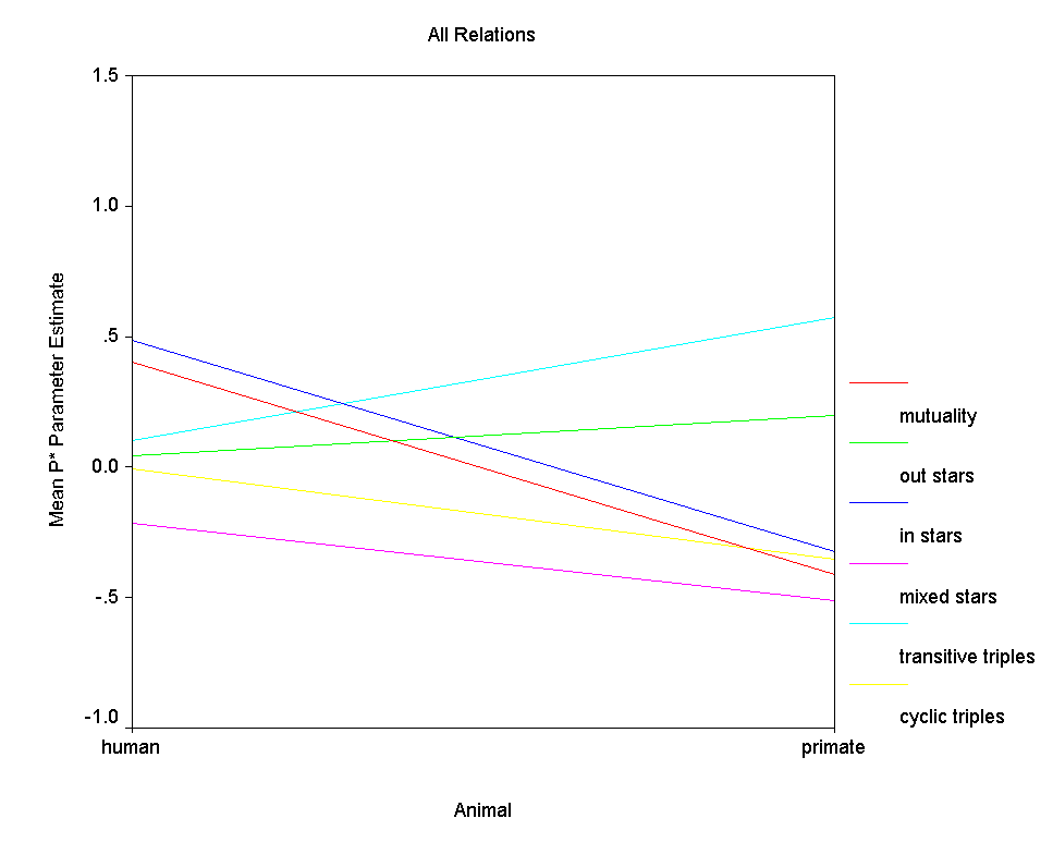
Figure 7.Ā Mean P* Parameter Estimates by Type of Animal
It is clear from the table and the figure that the mean
parameter values for human relations differ considerably from
those for primate relations for several structural effects except
for the out 2-stars effect.Ā Two differences are
particularly dramatic - the difference in mutuality and the
difference in in 2-stars.Ā The average level of mutuality
among human relations is a positive standardized coefficient
about .40 while the average level of mutuality among primate
relations is a negative standardized coefficient near .55.Ā
Among human relations, in 2-stars also has a positive effect but
among primate relations, the in 2-stars effect is just as
strongly negative.Ā This in 2-star effect captures how
important indegree variance is to the probability of a graph,
with positive values indicating graphs with relative more
indegree variance are more likely.Ā Thus indegree variance
contributes to graph probability among humans but detracts from
it among primates.Ā Less dramatic are the differences
between humans and primates in the transitive and cyclical triple
effects.Ā Among humans the average impact of both effects is
near .00, meaning that neither an abundance of cyclical triples
nor an abundance of transitive triples enhance graph probability
among humans.Ā However, among primates, the transitivity
effect is strongly positive while the cyclical triple effect is
modestly negative, indicating that graphs with many transitive
triples and few cyclical ones have higher probability.Ā
Finally, in both populations the effect of mixed 2-stars is
negative, meaning that in human and primate relations analyzed,
the tendency for nodes to be either sources of ties or targets of
ties, but not both, increases graph probability.
The Freeman-Linton hypothesis suggests that we now ask whether
these differences between the kinds of species arise because
different types of relations are measured in each.Ā For
instance, if negative, agonistic relations have strong transitive
and anti-cyclical tendencies (the dominance hierarchy effect),
then if the primate networks were disproportionately negative
ties and the human networks were disproportionately positive
ties, we would expect the average effects of transitive triples
and cyclical triples to be very different in the primate networks
than in the human networks.Ā Figures 8 and 9 graph the mean
parameter values separately for positive and negative relations
among humans vs. primates.Ā Figures 10-15 are box plots that
provide a more complete view of the overall distribution of
parameter values within kind of species by relation type.
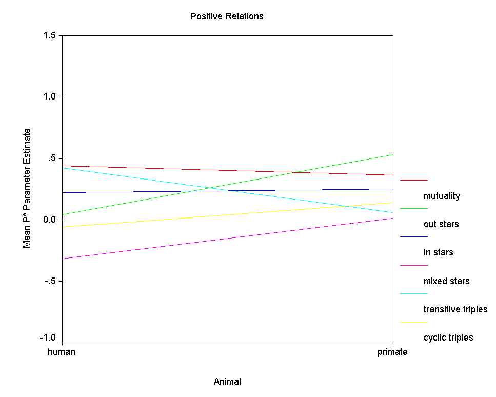
Figure 8.Ā Mean P* Parameter Estimates by Type of Animal
for Positive Relations
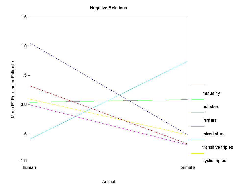
Figure 9.Ā Mean P* Parameter Estimates by Type of Animal
for Negative Relations
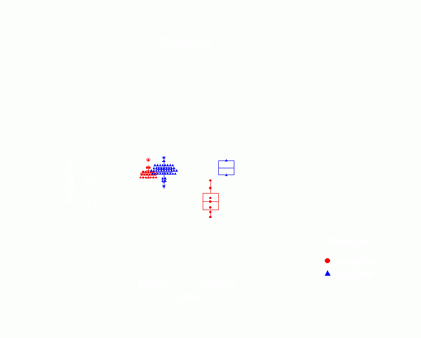
Figure 10.Ā Box Plot of Mutuality Parameters from p*
Model by Type of Animal
and Whether Relation is Positive or Negative
| Ā | |
| Ā | 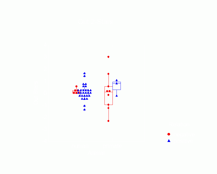
|
and Whether Relation is Positive or Negative
| Ā | |
| Ā | 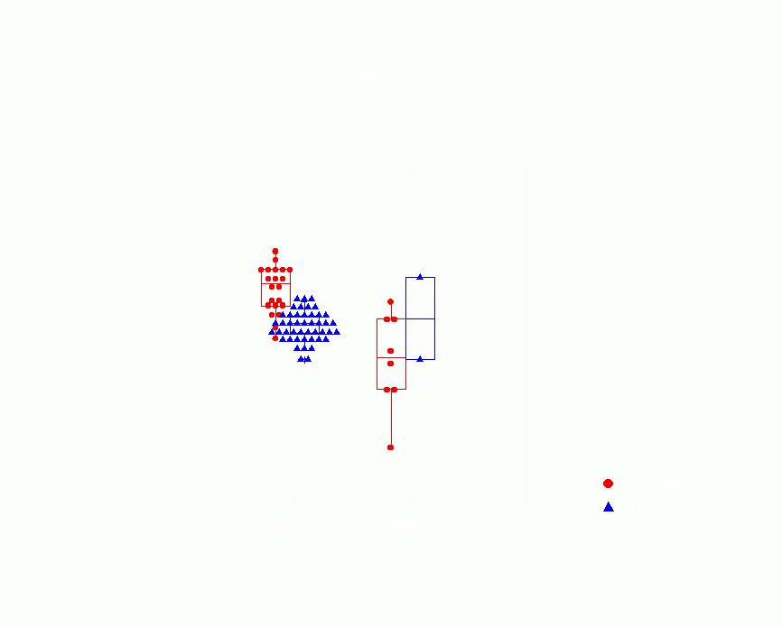 |
Figure 12.Ā Box Plot of In 2-Star Parameters
from p* Model by Type of Animal
and Whether Relation is Positive or Negative
 Figure
13.Ā Box Plot of Mixed 2-Star Parameters from p* Model by Type of Animal
and Whether Relation is Positive or Negative
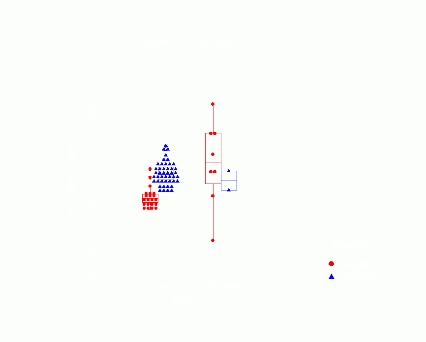 Figure 14.Ā Box Plot of Transitive
Triple Parameters from p* Model by Type of Animal
and Whether Relation is Positive or Negative
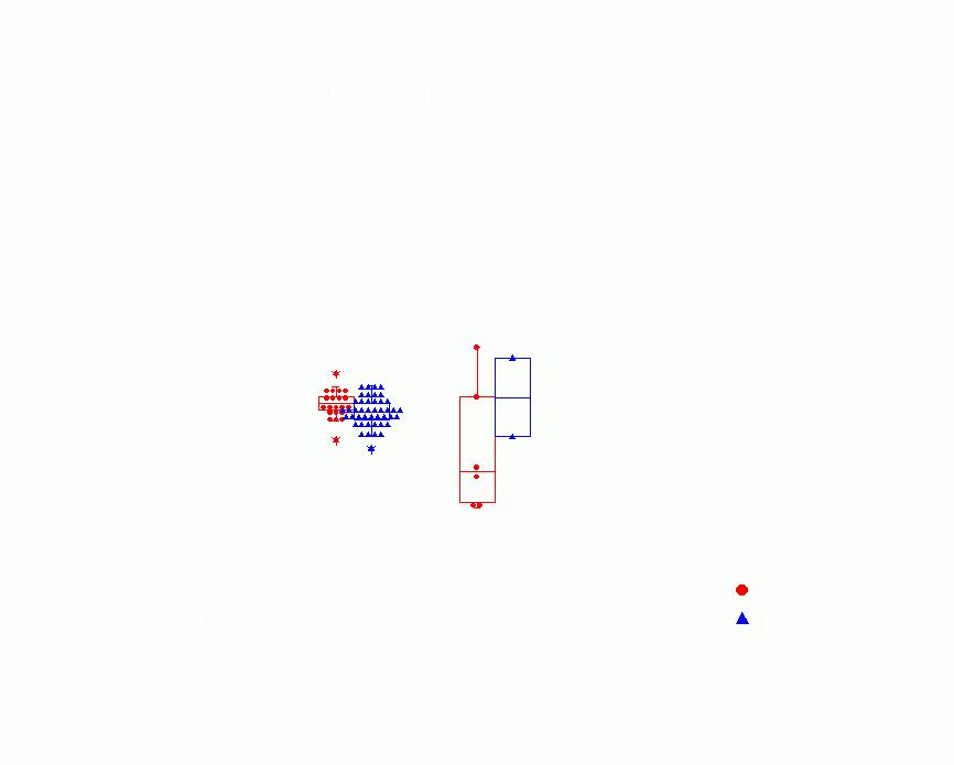 Figure 15.Ā Box Plot of Cyclic
Triple Parameters from p* Model by Type of Animal
and Whether Relation is Positive or Negative
Figure 8 clearly shows that positive relations are similarly structured among humans and among primates.Ā Perhaps the sole exception is with respect to the transitive triples effect, which is modestly positive in the human networks and absent completely in the positive primate networks.Ā However, since there are relatively few positive primate networks, small differences in average parameter value should not be over interpreted.Ā Figure 9, on the other hand, clearly shows that negative relations among humans are structured quite differently than negative relations among primates.Ā With the exception of the out 2-stars effect, the effects of the six structural factors differ considerably between the kinds of species.Ā First, negative relations tend to be modestly mutual among humans but to exhibit anti-mutuality among the primates.Ā Second, among primates many transitive triples of negative ties tend to enhance graph probability, while among humans, many would tend to depress graph probability.Ā Third, among human negative relations there is no effect of cyclical triples, while among primate negative relations, the effect is clearly negative, meaning that graphs with fewer cyclical triples have higher probability.Ā Human negative relations tend not to be transitive (nor particularly cyclical), while primate negative relations tend to be both transitive and anti-cyclical.Ā Fourth, the effect of in 2-stars on graph probability is strongly positive among humans but modestly negative among primates, meaning that indegree variance in negative relations contributes to graph probability among humans but depresses graph probability among primates.Ā Finally, there is no effect of mixed 2-stars among human negative relations, but there is a negative effect among primates.Ā That is, among primates nodes tend to be either sources or targets of negative ties, but not both.Ā
Overall then we must conclude that the
Freeman-Linton hypothesis is confirmed with respect to positive
relations but not with respect to negative relations.Ā That
is, species makes little difference in the "structural
signatures" of positive relations.Ā However, the
"structural signatures" of negative relations differ
substantively in many ways between humans and primates.Ā
Figures 16 and 17 graphically demonstrate the difference between
positive and negative relations.Ā Figure 16 is based on a
correspondence analysis of the distances between networks of
positive relations among humans and primates, and Figure 17, on
the distances between the negative relations.Ā Figure 17
clearly shows the separation between the kinds of species in two
dimensions.Ā The 68.2% confidence ellipses do not overlap at
all.Ā Figure 16 shows that the positive human networks are
embedded within the positive primate networks, the confidence
ellipse for the human networks is completely within that for the
primate networks.Ā Figure 16 also shows more research needs
to be done.Ā There are only three positive primate networks
and they are quite variable and so produce a very large
confidence ellipse.Ā Furthermore, they appear to lie on the
"outskirts" of the human positive networks although in
different directions from human networks' centroid.Ā The
pattern suggests that further research may find that the
Freeman-Linton hypothesis will not be sustained even for positive
relations.
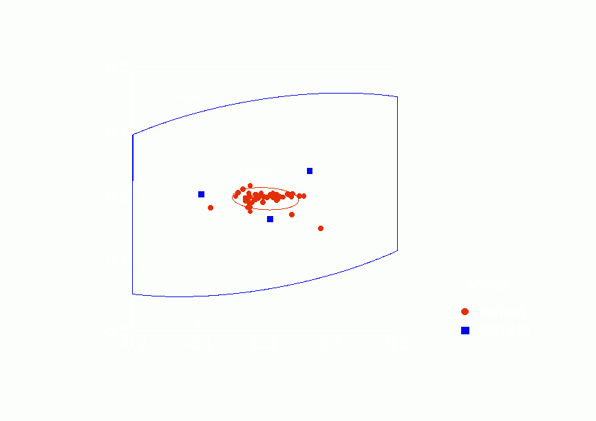 Figure 16.Ā
Confidence Ellipses for Type of Animal Overlaid on Correspondence Analysis of
Similarities between Positive Relations from p* Model Parameters, Column Scores
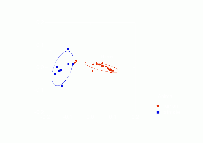 Figure 17.Ā
Confidence Ellipses for Type of Animal Overlaid on Correspondence Analysis of
Similarities between Negative Relations from p* Model Parameters, Column Scores
Ā
Discussion
The research we reported here had two aims:Ā first, to replicate and extend methodology for the comparison of networks first introduced in Faust and Skvoretz (forthcoming) and, second, to evaluate evidence bearing on what we called the "Freeman-Linton Hypothesis."Ā This hypothesis, suggested by observations of Linton Freeman and Ralph Linton, argues for no fundamental difference between the networks of relations among humans and the networks of relations among other primates or even among other nonprimate species.Ā More precisely stated, once relation type is taken into account, the networks are expected to be similarly structured, or in our terms, have similar "structural signatures."Ā To conclude, we comment on two points: the tenability of the Freeman-Linton hypothesis and its value to research, even if it appears to be difficult to find empirical confirmation, and the general theoretical importance of a research program that systematically compares networks.
The Freeman-Linton hypothesis fails to be confirmed with respect to negative relations in our collection of networks.Ā That is, negative relations among primates have significantly different structural signatures than negative relations among humans.Ā How seriously should we take this disconfirmation?Ā If we knew that the nature of the behavior defining the connections was common to both networks, we would be forced to abandon the hypothesis.Ā But, of course, we do not know this for a fact -- indeed, can never know it for a fact.Ā Rather, the disconfirmation forces us to probe more deeply into the difference between the behaviors defining the negative relational networks in humans and the behaviors defining the negative relations among primates.Ā There is a difference.Ā Among primates, the negative ties are generated by success in agonistic encounters, conflictual interactions with winners and losers.Ā Among humans, most of the negative ties in our collection are generated by questions about the respondents' feelings towards others:Ā do they dislike or hold in low esteem other group members.Ā This indicator is neither behavioral nor "zero-sum" in the way an agonistic encounter is.Ā Given the ties we have analyzed, it is thus not surprising that negative relations among primates differ from those among humans once we realize just how different the ties are in behavioral contents.Ā Therefore, if we had networks among humans based on success in agonistic encounters, we expect that they would have very similar structural signatures to our negative networks among primates.[5]Ā On the other hand, if we had networks based on avowed disliking or disesteem among primates, we expect that they would have structural signatures similar to our negative networks among humans.
We argue that the real value of the Freeman-Linton hypothesis lies not in whether it is empirically supported, but in its use as a tool to refine the conceptual categories by which we classify modes of social relatedness.Ā Empirical disconfirmation of the hypothesis, which we face in the current work, is a spur to more carefully delineate the fundamental dimensions along which social ties differ.Ā In the current research we have used rather crude classifications based on the valence of the tie, positive or negative, and on how data defining the tie were collected, by observation or by respondent report.Ā Even though this classification scheme is rough-cut, it still helps us to order the data on the 80 networks in a consistent fashion.Ā But it does not provide a complete account and thus supplies an impetus for further research based on more refined classification schemes.
Methodological concerns drive the current project's comparison of networks.Ā Our primary interest is the mechanics of how such a comparison might be accomplished, particularly, when the networks vary substantially in size, in relational type, and in species over which the relation is defined.Ā Yet the results create a theoretical agenda by raising questions about the theoretical reasons for similarities and differences in the structural signatures of networks.Ā We can illustrate this point with some examples.Ā
Consider, for instance, the studies of work groups that often ask about the advice network among co-workers, that is, who goes to whom for advice.Ā Selection of advice seeking as an important social tie may have its roots in Peter Blau's early study of advice-seeking in a bureaucracy as a social exchange phenomenon (Blau 1955).Ā Theoretically, one might argue that the nature of the advice seeking relation is revealed in the structural properties that affect the probability of particular graphs of the advice relation.Ā Thus we might expect advice networks in different organizational settings to have similar structural signatures.Ā Empirical research may reveal some commonalities but also some variants, thus establishing a problem for theory:Ā what accounts for the commonalities, that is, an articulation of what is the "nature" of the advice seeking relation, and what accounts for its variants, for instance, the advice relation may differ in characteristic ways across cultures or across organizational forms or industries.
Further, the comparison of the structural signature of advice relations with other types of relations, such as friendship, may help illuminate the social and social psychological principles that differentiate such ties.Ā Clearly, the populations we study recognize such ties as different.Ā As researchers, we "know" such ties are different if for no other reason than that they, typically, link up different pairs of persons in our study population.Ā But to account for these differences and to even consider how to measure such differences are tasks that have not been as high on the social network research agenda as they perhaps should be.Ā Attention to these issues should give us a deeper understanding of the range and analytical types of relatedness among individuals.
Other territory opened for exploration would be any theoretical studies for which "ideal" types of networks are important conceptualizations in the theoretical enterprise.Ā An example here is the work of Markovsky (1998) on solidarity.Ā Markovsky hypothesizes that the solidarity of a group in terms of the network of communication ties among group members depends on the nature of the group.Ā Different types of groups have different "referent" networks against which their solidarity should be calibrated.Ā In Markovsky's thinking, a referent network is a pattern of actors and ties that identifies a class of networks.Ā He gives as an example a "cult" in which the referent network is "ten or more followers, each with ties of adoration and social attachment directed toward a leader, and each with ties to at least one other follower" (Markovsky 1998: 357).Ā The solidarity of a group depends on the extent to which its interaction pattern approximates the referent pattern for its type.Ā This conceptualization is, clearly, comparative:Ā to assess the solidarity of cult X we need to compare its interaction pattern with the referent pattern.Ā Our idea of "structural signatures" clarifies the nature of the comparison and says that the solidarity of cult X is measured by the similarity in the structural signatures of cult X and the cult referent-network.Ā Furthermore, the idea of structural signatures permits measuring degrees of solidarity - that is, the extent to which cult X approximates the ideal pattern.
These theoretical dimensions to the comparison problem are independent of the specific methodology by which networks are compared.Ā These questions could have been asked several decades ago, but the answers, that is, the profile of structural effects that could be incorporated into the signature, were very limited.Ā Advances in the statistical modeling of networks have made it possible to expand vastly the elements composing a network's structural signature.Ā Yet we must recognize that this expansion is not the end of the story.Ā Future advances in statistical modeling will make the identification of a network's structural signature ever more precise.Ā There is no doubt that more precision will improve upon and possibly change the findings we have reported.Ā But more precision will not nullify the importance of the theoretical issues that network comparisons address.
One final issue of theoretical importance as it bears on the evaluation of hypotheses is whether our sample of networks represents a complete range of typical social relations.Ā Without a definition of the "population" of social relations our sample is to represent, it is clear that we cannot answer this question.Ā It appears that many kinds of relations are underrepresented in our sample, including both affectionate and agonistic behavioral encounters among humans and affectionate encounters among nonhuman primates and nonprimate mammals.Ā The extent to which a non-representative sample of relational contents might lead to an incorrect conclusion about the Freeman-Linton hypothesis (or about any other hypothesis about the basis for commonalities among network structures) is worthy of further investigation.
Ā
References
Anderson, Carolyn J., Stanley Wasserman, and Bradley Crouch.Ā 1999.Ā "A p* primer: Logit models for social networks."Ā Social Networks 21: 37-66.
Bernard, H. Russell, Peter Killworth, and Lee Sailer. 1980. "Informant Accuracy in Social Network Data IV: A Comparison of Clique-Level Structure in Behavioral and Cognitive Network Data."Ā Social Networks 2, 191-218.
Blau, Peter M.Ā 1955.Ā The Dynamics of Bureaucracy.Ā Chicago:Ā University of Chicago Press.
Burt, Ronald.Ā 1991.Ā Structure 4.2.Ā Center for the Social Sciences, Columbia University.
Carroll, J. Douglas, Ece Kumbasar, and A. Kimball Romney.Ā 1997.Ā "An Equivalence Relation between Correspondence Analysis and Classical Multidimensional Scaling for the Recovery of Euclidean Distances."Ā British Journal of Mathematical and Statistical Psychology 50: 81-92.
Coleman, James.Ā 1964.Ā Introduction to Mathematical Sociology.Ā New York: Free Press.
Crouch, Bradley, and Stanley Wasserman.Ā 1998.Ā "A Practical Guide to Fitting p* Social Network Models."Ā Connections 21: 87-101.
Dunbar, R. I. M., and E. P. Dunbar.Ā 1976.Ā "Contrasts in Social Structure among Black-and-White Colobus Monkey Groups."Ā Animal Behaviour, 24: 84-92.
Faust, Katherine, and John Skvoretz.Ā Forthcoming.Ā "Comparing Networks Across Space and Time, Size and Species." ĀSociological Methodology, forthcoming.
Frank, O., and D. Strauss.Ā 1986.Ā "Markov Graphs."Ā Journal of the American Statistical Association 81: 832-842.
Freeman, Linton.Ā 1999.Ā "Research in Social Networks."ĀAvailable: http://eclectic.ss.uci.edu/~lin/work.html [June 18, 2002].
Freeman, Sue C., and Linton C. Freeman. 1979. The Networkers Network: A Study of the Impact of a New Communications Medium on Sociometric Structure. Social Science Research Reports, No. 46. Irvine, CA: University of California.
Friedkin, Noah E.Ā 1998.Ā A Structural Theory of Social Influence.Ā Cambridge, UK: Cambridge University Press.
Hall, K.R. L., and Irven DeVore.Ā 1965. "Baboon Social Behavior."Ā Pp. 53-110 in Primate Social Behavior: Field Studies of Monkeys and Apes, edited by Irven DeVore.Ā New York: Holt, Rinehart, and Winston.
Hausfater, Glenn.Ā 1975.Ā Dominance and Reproduction in Baboons (Papio cynocephalus), a Quantitative Analysis.Ā New York: S. Karger.
Kapferer, Bruce. 1972. Strategy and Transaction in an African Factory: African Workers and Indian Management in a Zambian Town. Manchester: Manchester University Press.
Katz, L., and J.H. Powell.Ā 1955.Ā "Measurement of the Tendency toward Reciprocation Choice."Ā Sociometry 19: 403-409.
Katz, L., and T.R. Wilson.Ā 1956.Ā "The Variance of the Number of Mutual Choices in Sociometry."Ā Psychometrika 21: 299-304.
Krackhardt, David.Ā 1987. "Cognitive Social Structures."Ā Social Networks 9: 104-134.
_____.Ā 1988.Ā "Predicting with Networks:Ā Nonparametric Multiple Regression Analyses of Dyadic Data."Ā Social Networks 10: 359-382.
Linton, Ralph.Ā 1936.Ā The Study of Man.Ā New York: The Free Press.
MacRae, Duncan.Ā 1960. "Direct Factor Analysis of Sociometric Data."Ā Sociometry 23: 360-371.
Mandel, Micha.Ā 2000.Ā "Measuring Tendency towards Mutuality in a Social Network."Ā Social Networks 22: 285-298.
Markovsky, Barry.Ā 1998.Ā "Social Network Conceptualizations of Solidarity."Ā Pp. 343-372 in "The Problem of Solidarity:Ā Theories and Models" edited by Patrick Doreian and Thomas Fararo.Ā Amsterdam, The Netherlands:Ā Gordon and Breach.
McGrew, W. C. 1972.Ā An Ethological Study of Children's Behavior.Ā New York: Academic Press.
Newcomb, Theodore. 1961. The Acquaintance Process. New York: Holt, Reinhardt andWinston.
Parker, J. G. and S. Asher.Ā 1993.Ā "Friendship and Friendship Quality in Middle Childhood" Links with Peer Group Acceptance and Feelings of Loneliness and Social Dissatisfaction."Ā Developmental Psychology 29: 611-621.
Pattison, Philippa, and Stanley Wasserman.Ā 1999.Ā "Logit models and logistic regressions for social networks: II.Ā Multivariate relations."Ā British Journal of Mathematical and Statistical Psychology 52: 169-193.
Pattison, Philippa, Stanley Wasserman, Garry Robins, and Alaina Michaelson Kanfer. 2000.ĀĀ "Statistical Evaluation of Algebraic Constraints for Social Networks."Ā Journal of Mathematical Psychology 44: 536-568.
Robins, Garry, Philippa Pattison, and Stanley Wasserman.Ā 1999.Ā "Logit Models and Logistic Regressions for Social Networks: III.Ā Valued Relations."Ā Psychometrika 64: 371-394.
Sade, Donald S. 1967.Ā "Determinants of Dominance in a Group of Free-ranging Rhesus Monkeys."Ā Pp. 99-114 in Social Communication among Primates edited by Stuart A. Altmann.Ā Chicago: University of Chicago Press.
Sampson, Samuel F. 1968.Ā A Novitiate in a Period of Change: An Experimental and Case Study of Social Relationships.Ā Unpublished doctoral dissertation.Ā Cornell University.
Schein, Martin W., and Milton H. Fohrman.Ā 1955.Ā "Social Dominance Relationships in a Herd of Dairy Cattle."Ā The British Journal of Animal Behavior 3: 45-55.
Strauss, David, and Michael Ikeda.Ā 1990.Ā "Pseudolikelihood Estimation for Social Networks."Ā Journal of the American Statistical Association 85: 204-212.
Strayer, F. F., and Janet Strayer.Ā 1976.Ā "An Ethological Analysis of Social Agonism and Dominance Relations among Preschool Children." Child Development 47: 980-989.
Tyler, Stephanie J.Ā 1972.Ā "The Behaviour and Social Organization of the New Forest Pony."Ā Animal Behavior Monographs, Volume 5, Part 2.
Vickers, M., and S. Chan. 1981.Ā Representing Classroom Social Structure.Ā Melbourne: Victoria Institute of Secondary Education.
Wasserman, Stanley, and Philippa Pattison. 1996. "Logit Models and Logistic Regressions for Social Networks: I. An Introduction to Markov Graphs and p*."Ā Psychometrika 61: 401-425.
Ā
Appendix:Ā List of Data Sources
This appendix lists the 80 networks, describes the relations, gives a reference for the source of the data, and reports the label used in tables and figures.Ā Where data are published, the table number and page of the source are given.
- baboonf: dominance interactions between female and one adult male baboons (Figure 3-8, page 69, Hall and DeVore 1965)
- baboonm1 and baboonm2: dominance between male baboons (Table 3-2, page 60, Hall and DeVore 1965)
- baboonm3:Ā outcomes of agonistic bouts between male baboons (Table XI, page 39, Hausfater 1975)
- banka:Ā advice in a bank office (Table 5, page 558, Pattison et al. 2000)
- bankc: confiding in a bank office (Table 5, page 558, Pattison et al.2000)
- bankf:Ā close friends in a bank officeĀ (Table 5, page 558, Pattison et al.2000)
- banks:Ā satisfying interaction in a bank officeĀ (Table 5, page 558, Pattison et al.2000)
- bkfrac:Ā rating of interaction frequency in a fraternity.Ā Originally coded 1 - 5; recoded 4,5 =1, <4=0.Ā (Appendix A, Bernard, Killworth, and Sailer 1980, also available in UCINET, Borgatti, Everett, and Freeman 1999)
- bkhamc:Ā rating of interaction frequency between ham radio operators. Originally coded 1 - 9; recoded 7,8,9 =1, <7=0 (Appendix A, Bernard, Killworth, and Sailer 1980, also available in UCINET, Borgatti, Everett, and Freeman 1999)
- bkoffc:Ā top rank order of interaction frequency in an office. Originally a complete rank order from 1 to 39; recoded 1-13=1, >13=0.Ā (Appendix A, Bernard, Killworth, and Sailer 1980, also available in UCINET, Borgatti, Everett, and Freeman 1999)
- bktecc:Ā top rank order of interaction frequency in a technical group.Ā Originally a complete rank order from 1 to 36; recoded 1-11=1, >11=0.Ā (Appendix A, Bernard, Killworth, and Sailer 1980, also available in UCINET, Borgatti, Everett, and Freeman 1999)
- camp92:Ā top rank order of interaction frequency in "Camp". Originally a complete rank order from 1 to 17, recoded 1-6=1, >6=0. (available in UCINET, Borgatti, Everett, and Freeman 1999)
- cattle:Ā contests between dairy cattle (Figure 1, page 49, Schein and Fohrman 1955)
- cole1:Ā friendship at time 1 between high school boys (Table 14.5 (a), page 450, Coleman 1964)
- cole2: friendship at time 2 between high school boys (Table 14.5 (b), page 451, Coleman 1964)
- colobus1:Ā non-agonistic social acts between colobus monkeys in a small group (Table I, page 86, Dunbar and Dunbar 1976)
- colobus2:Ā non-agonistic social acts between colobus monkeys in a small group (Table I, page 86, Dunbar and Dunbar 1976)
- colobus4:Ā non-agonistic social acts between colobus monkeys in a large group (Table II, page 87, Dunbar and Dunbar 1976)
- eiesk1:Ā EIES data, rating of acquaintanceship.Ā Recoded 3,4=1, <3=0. (Freeman and Freeman 1979; Table B.8, page 745, Wasserman and Faust 1994)
- eiesk2:Ā EIES data, rating of acquaintanceship.Ā Recoded 3,4=1, <3=0. (Freeman and Freeman 1979; Table B.9, page 746, Wasserman and Faust 1994)
- eiesm:Ā EIES data frequency of message sending, Recoded "1" if any message was sent. (Freeman and Freeman 1979; Table B.10, page 747,Wasserman and Faust 1994)
- fifth:Ā friendships between fifth graders (Table 3, page 44, Anderson et al. 1999, data from Parker and Asher 1993)
- fourth: friendships between fourth graders (Table 3, page 44, Anderson et al. 1999, data from Parker and Asher 1993)
- ka: Each manager was asked who they went to for help or advice at work. (Krackhardt 1987;ĀĀ Data available in Wasserman and Faust 1994 and UCINET, Borgatti, Everett, and Freeman 1999).
- kapfti1: instrumental work relations in a tailor shop, time 1 (Matrix 1, pages 176-177, Kapferer 1972)
- kapfti2:Ā instrumental work relations in a tailor shop, time 2 (Matrix 2, pages 178-179, Kapferer 1972)
- kf:Ā Each manager was asked who they were friends with at work. (Krackhardt 1987;ĀĀ Data available in Wasserman and Faust 1994 and UCINET, Borgatti, Everett, and Freeman 1999).
- kids1:Ā initiated agonism between children (Figure 2, page 986, Strayer and Strayer 1976)
- kids2: dominance among boys in a nursery school (Figure 5.5, page 125, McGrew 1972)
- medical: ties between physicians (Coleman, Katz and Menzel, data available in Structure, Burt 1991) newc0 to newc15:Ā top rankings of friendship in a fraternity, weeks 0 through 15.Ā Original data were complete rank orders, recoded 1-5=1, >5 = 0.Ā (Newcomb 1961, data available in UCINET, Borgatti, Everett, and Freeman 1999).
- newc0n to newc15n:Ā bottom rankings of friendship in a fraternity, weeks 0 through 15.Ā Original data were complete rank orders; recoded 11-15=1, <11 = 0 (Newcomb 1961, data available in UCINET, Borgatti, Everett, and Freeman 1999).
- nfponies: threats between ponies (Table XIV, page 122, Tyler 1972)
- prison:Ā closest friendships in a prison (Table 1, page 363, MacRae 1960)
- rhesus1:Ā fights between adult female rhesus monkeys (Table 1, page 105, Sade 1967)
- rhesus2:Ā fights between yearling rhesus monkeys (Table 2, page 107, Sade 1967)
- rhesus4:Ā fights between adult rhesus monkeys (Table 4, page 108, Sade 1967)
- rhesus5:Ā fights between adult rhesus monkeys (Table 7, page 110, Sade 1967)
- rhesus6: fights between adult rhesus monkeys (Table 8, page 111, Sade 1967)
- sampdes:Ā disesteem between monks, time 4 (Table D14, page 470, Sampson 1968)
- sampdlk:Ā dislike between monks in a monastery, time 4 (Table D13, page 469, Sampson 1968, available in UCINET, Borgatti, Everett, and Freeman 1999)
- sampes:Ā esteem between monks in a monastery,Ā time 4 (Table D14, page 470, Sampson 1968, available in UCINET, Borgatti, Everett, and Freeman 1999)
- sampin:Ā influence between monks in a monastery, time 4 (Table D15, page 471, Sampson 1968, available in UCINET, Borgatti, Everett, and Freeman 1999)
- samplk:Ā liking between monks in a monastery, time 4 (Table D13, page 469, Sampson 1968, available in UCINET, Borgatti, Everett, and Freeman 1999)
- sampnin:Ā negative influence between monks in a monastery,Ā time 4 (Table D15, page 471, Sampson 1968, available in UCINET, Borgatti, Everett, and Freeman 1999)
- sampnpr: negative praise (blame) between monks in a monastery,Ā time 4 (Table D16, page 471, Sampson 1968, available in UCINET, Borgatti, Everett, and Freeman 1999)
- samppr:Ā praise between monks in a monastery,Ā time 4 (Table D16, page 471, Sampson 1968, available in UCINET, Borgatti, Everett, and Freeman 1999)
- third:Ā friendship between third graders (Table 1, page 42, Anderson et al.1999, data from Parker and Asher 1993)
- vcbf:Ā best friends between seventh graders (Table 3, page 385, Robins, Pattison, and Wasserman 1999, from Vickers and Chan 1981)
- vcg:Ā get on with between seventh graders (Table 11, page 422, Wasserman and Pattison 1996, from Vickers and Chan 1981)
- vcw:Ā work with between seventh gradersĀĀ
(Table 12, page 423, Wasserman and Pattison 1996, from
Vickers and Chan 1981)
Footnotes
[1] In our analysis, as in Faust and Skvoretz (forthcoming) we use the p* modeling framework to estimate the collection of parameters comprising the structural signature of each network.Ā This is by no means the only possible approach, but it has several advantages as compared to other approaches currently available.Ā In general the problem is to express, for each network, its structural tendencies.Ā Obviously there are numerous graph theoretic properties that could be used for this characterization.Ā One problem is to express these tendencies in a "metric" that is comparable across networks of different scale (different sizes and densities).Ā Using standardized regression coefficients from the statistical model accomplishes this by expressing the effect of a structural property in standardized units, and does so for all properties and all graphs. This facilitates comparison across networks.Ā A second problem is possible interdependencies among structural properties.Ā For example, an observed level of transitivity in a graph might be attributable to the graph's high density or tendency for mutuality.Ā Using a statistical model which estimates effects of structural parameters simultaneously deals with this by expressing the effect of a structural property, net of other factors in the model.Ā Certainly other statistical models (such as Friedkin's (1998) local density model) or quantifications of structural properties are possible avenues for constructing structural signatures.
[2]Ā However, using such routines assumes, contrary to fact, that the logits are independent.Ā Therefore, the model is not a true logistic regression model and statistics from the estimation must be used with caution.Ā Goodness of fit statistics are pseudo-likelihood ratio statistics, it is questionable whether the usual chi-square distributions apply, and standard errors only have "nominal" significance (see Crouch and Wasserman 1998).
[3] Given the pseudo-likelihood estimation underlying the p* model, we need to be cautious about literal interpretation of the parameter estimates, particularly when they attain extreme values.Ā While we look at means of subsets of estimates to compare structural tendencies between different kinds of networks, the reader should be aware that extreme values are suspect.Ā However, such comparison are the best we can do until there are better models and estimation techniques.
[4]Ā Among humans, it was possible to estimate the full model in 33 of the 66 networks.Ā In the other 33, a model with five parameters could be estimated.Ā Among primates, the full model could be estimated in six of the 12 networks, a model with five parameters in two, a model with four in two, and a model with only two parameters in the remaining two networks.Ā The two mammal networks allowed for the estimation of the full model in one and a model with four parameters in the other.
[5]Ā There is some support for this speculation.Ā We have two networks of observed negative encounters between humans - initiated agonism among nursery school boys (labeled kids1 and kids2, respectively).Ā In Figure 2, these networks areĀ in the lower left corner of the plot.Ā They are situated on the lower edge of the networks of observed negative encounters among primates and mammals (on the left of the figure) and are clearly separated from the negative affective ties among humans (on the right of the figure).
