Eigen Analysis of Networks
William Richards and Andrew Seary
School of Communication, Simon Fraser University
Burnaby, BC Canada
[This article is published jointly by Structural Analysis and Journal of Social Structure.]
ABSTRACT: We present an overview of eigen analysis methods and their applications to network analysis. We consider several network analysis programs/procedures (Correspondence Analysis, NEGOPY, CONCOR, CONVAR, Bonacich centrality) that are at their core eigendecomposition methods. We discuss the various matrix representations of networks used by these procedures and we give particular attention to a variety of centering and normalizing procedures that are carried out prior to the analysis. We compare three types of iterative procedures with the standard SVD in terms of pragmatic concerns and the results produced by each method. We show how the initial matrix representations and the adjustments made between iterations influence the results obtained. Finally, we show that the eigen perspective clearly highlights the similarities and differences between different network analysis procedures.
Introduction
We consider several network analysis programs/procedures that are at their core eigendecomposition methods. These include Correspondence Analysis (CA), NEGOPY, CONCOR, CONVAR, Bonacich centrality. We describe the procedures these analytic approaches use and consider these procedures from a variety of perspectives. We consider the results produced by the various approaches and examine the similarities and differences between them in terms of what they tell the user about networks and what it is about the procedures that is the source of the strengths and weaknesses of the methods.
Network Analysis and Eigendecomposition
Network analysis begins with data that describes the set of relationships among the members of a system. The goal of analysis is to obtain from the low-level relational data a higher-level description of the structure of the system. The higher-level description identifies various kinds of patterns in the set of relationships. These patterns will be based on the way individuals are related to other individuals in the network. Some approaches to network analysis look for clusters of individuals who are tightly connected to one another (clique detection); some look for sets of individuals who have similar patterns of relations to the rest of the network (structural equivalence).
Other methods don't "look for" anything in particular -- instead, they construct a continuous multidimensional representation of the network in which the coordinates of the individuals can be further analyzed to obtain a variety of kinds of information about them and their relation to the rest of the network. One approach to this is to choose a set of axes in the multidimensional space occupied by the data and rotate them so that the first axis points in the direction of the greatest variability in the data; the second one, perpendicular to the first, points in the direction of greatest remaining variability, and so on. This set of axes is a coordinate system that can be used to describe the relative positions of the set of points in the data. Most of the variability in the locations of points will be accounted for by the first few dimensions of this coordinate system. The coordinates of the points along each axis will be an eigenvector, and the length of the projection will be an eigenvalue.
Researchers who use methods like Correspondence Analysis or principle components analysis are generally aware that they are using eigen decomposition methods. Those who use computer programs such as CONCOR or NEGOPY, however, may not be aware of this because the eigenvalues or eigenvectors are hidden more or less deeply within the analytic package. Nevertheless, eigen methods lie at the heart of these analytic tools.
Network researchers have used eigen decomposition methods either implicitly or explicitly since the late 1960's, when computers became generally accessible in most universities. In the last twenty years there has been an increasing use of these methods which have become available on microcomputers.
The simplest approach to eigen analysis is to submit the adjacency matrix to SVD (singular value decomposition) or a standard eigen decomposition routine. This will result in a set of eigenvectors and eigenvalues that we refer to here as the "Standard" spectrum of the network. The Bonacich eigenvector is the first one in the set -- the one associated with the largest eigenvalue. Because this approach begins with the raw adjacency matrix and does not deal with expected (based on row and/or column marginals) effects, the results contain a mixture of "signal" and "background" and are thus difficult to interpret.
Correspondence Analysis (CA) begins by dividing the elements of the
adjacency matrix by the sum of all the elements in the matrix. This
normalized matrix, C, is processed as in the calculation of chi-squared. CA is essentially eigen decomposition of the square root of the ![]() matrix (C - E)2/E where E is the matrix of expected values of C,
and the eigenvectors are weighted by the reciprocal of the square root
of the marginals (Greenacre, 1984; Hoffman & Franke, 1986). The
result of the eigen decomposition is a set of eigenvectors and
eigenvalues that we refer to here as the "Normal" spectrum of the
network. The first n-1 eigenvectors describe the
"signal" that remains after subtracting the "background" expected
eigenvector, weighted by the eigenvalues. The last eigenvector is
weighted by 0.0, and is called the "trivial" eigenvector. It
corresponds to the expected values, and plays no further part in CA.
Some researchers add the row sums (or some other number) to the
corresponding diagonal elements of the adjacency matrix before
normalizing. This "balancing" shifts the eigenvalues so the negative
ones become positive. This procedure has important consequences which
are discussed in detail in a later section.
matrix (C - E)2/E where E is the matrix of expected values of C,
and the eigenvectors are weighted by the reciprocal of the square root
of the marginals (Greenacre, 1984; Hoffman & Franke, 1986). The
result of the eigen decomposition is a set of eigenvectors and
eigenvalues that we refer to here as the "Normal" spectrum of the
network. The first n-1 eigenvectors describe the
"signal" that remains after subtracting the "background" expected
eigenvector, weighted by the eigenvalues. The last eigenvector is
weighted by 0.0, and is called the "trivial" eigenvector. It
corresponds to the expected values, and plays no further part in CA.
Some researchers add the row sums (or some other number) to the
corresponding diagonal elements of the adjacency matrix before
normalizing. This "balancing" shifts the eigenvalues so the negative
ones become positive. This procedure has important consequences which
are discussed in detail in a later section.
NEGOPY uses an iterative method that converges to the same eigenvector produced by balanced CA. However, the process is stopped after only four to eight iterations, at which point the result contains a mixture of the most important positive eigenvectors which makes cohesive clusters of nodes relatively easy to identify.
CONVAR is the iterated calculation of covariance of pairs of rows (or columns) of the adjacency matrix. When successive rounds of calculations no longer produce different results, the process has converged to an eigenvector/eigenvalue pair whose components almost always have the same sign as those of the corresponding Standard pair. CONCOR is the iterated calculation of the Pearson correlation of pairs of rows (or columns) of the adjacency matrix. When successive rounds of calculations no longer produce different results, the process has converged. At this point, all correlations will be 1 or -1. Although it is very closely related to CONVAR, this method is not an eigen decomposition: it does not produce eigenvectors or eigenvalues.
There are several approaches to eigen analysis. They vary in two
important ways. First, they use different forms of the data which
describes the network. Some use the raw adjacency matrix while others
use an adjacency matrix that has been transformed. Many of these
transformations involve some kind of normalization or the removal of
one or more types of "expecteds." Because of these various
transformations, the analytic results provide different kinds of
information about the network. This issue is discussed further in later
sections of the paper. The second way in which the approaches differ is
the manner in which the actual eigen decomposition is accomplished.
There are four methods: direct application of an SVD routine to the
matrix, multiplying the matrix by itself until the result converges
(the power method), multiplying the matrix by a vector until the result
converges (a variant of the power method), and iteratively performing a
calculation, such as Pearson's r or covariance on the
matrix. As the following paragraphs point out, each of the various
approaches has its own strengths and weaknesses. There are two main
factors here: 1) the size of the network that can practically be
analyzed: some computational approaches require a great deal more
memory than others and are thus limited to the size of network they can
handle; and 2) the number of eigenvectors and eigenvalues the
researcher requires: ordinary eigendecomposition routines deliver all of the eigenvectors and eigenvalues, while the iterative approaches deliver only one eigenvector/eigenvalue pair at a time and require additional computational work to provide more.
Some methods of eigen analysis work by means of a direct analytic procedure in which a set of equations are used to directly calculate an exact result. Others use an iterative procedure that (hopefully) converges to an acceptable solution. Iterative methods for the extraction of eigenvectors take one of two forms, the power method and iterated calculation. We discuss the ordinary power method, two types of iterated calculations, and a variant of the power method that can be used for very large networks. In the discussion of these iterative procedures, we indicate the strengths and weaknesses of each. Throughout, we use the Sampson data (Figure 1) as an illustration.
|
0 1 1 0 1 1 0 0 0 0 0 0 0 1 1 0 0 0 1 0 0 1 1 1 1 1 0 1 0 0 0 1 1 0 0 0 1 0 0 0 0 0 0 0 1 1 0 0 0 0 0 0 0 1 0 1 0 0 0 0 0 1 0 0 0 0 0 0 0 0 0 1 1 1 0 0 0 0 1 0 0 0 0 0 0 0 1 0 0 0 1 1 0 0 0 0 1 0 0 0 0 0 0 0 0 0 0 0 0 1 0 0 1 1 0 1 0 0 0 0 0 0 0 0 0 0 0 1 0 1 0 0 1 0 0 0 0 0 0 0 0 0 0 0 0 0 1 0 0 0 0 0 0 1 0 0 0 0 0 0 0 0 0 1 1 0 0 0 0 0 1 0 0 0 0 0 0 0 0 1 0 0 0 0 0 0 0 0 0 0 0 1 1 1 1 1 1 0 0 0 0 0 0 0 0 0 0 0 1 0 0 0 0 0 1 1 0 0 0 0 0 0 0 0 0 0 1 0 0 1 1 0 1 0 1 1 0 0 0 0 0 0 0 0 1 0 1 0 1 0 1 0 1 1 0 0 1 0 0 0 0 0 1 0 1 1 0 0 1 0 0 0 0 0 0 0 0 0 0 0 1 0 0 0 0 0 0 1 0 0 0 0 0 0 0 0 0 0 1 1 1 1 1 0 0 1 0 0 1 1 0 0 0 0 0 1 0 1 0 0 0 1 1 0 |
| Figure 1.ĀĀ The Sampson data. |
Some useful facts about eigenvectors and eigenvalues will assist in the following discussion:
- The eigenvectors of X + cI (where c is a constant, and I is an identity matrix) are the same as the eigenvectors of X. In other words, adding a constant, c, to the diagonal elements of X does not affect the eigenvectors. However, the eigenvalues of X + c I are shifted by an amount equal to c. If the value 2.0 is added to all the diagonal elements of the matrix X, the eigenvalues will each be increased by 2.0.
- The eigenvalues of cX are c times the eigenvalues of X. In other words, if all elements of the matrix X are multiplied by a constant, the eigenvalues are also multiplied by the same constant. For example, the eigenvalues of -X are -(the eigenvalues of X).
- Taking powers of a matrix does not affect the eigenvectors; the eigenvalues are raised to the same power.
A. Power Method I: Naive Method
If an adjacency matrix for a connected network that is not bipartite is raised to higher and higher powers, it will eventually converge so that the columns will be multiples of one another and of the eigenvector that belongs to the largest eigenvalue that would be produced by an SVD of the adjacency matrix, which will be positive and unique.
There are a few problems with this naive power method:
- If the largest positive eigenvalue is not exactly equal to 1.0 (a
very likely case), the numbers in the matrix get either larger or
smaller with each multiplication as higher powers are calculated. For
example, with the Sampson data, the largest values in the matrix for
the first seven iterations are: 9, 661, 46050, 2930170, 184975591,
11675328497, and 737051615336. Very large and very small numbers can be
difficult to work with and are likely to reduce the level of accuracy
of the results.
- Because the values continue to get larger (or smaller) with
each iteration, it is necessary to perform some additional calculations
after each new power of the matrix to determine whether or not the
process has "converged." If the numbers in each column of the matrix
are divided by the column total, the result can be compared from
iteration to iteration. To make it easier to see when the process has
converged, the sum of the squared differences from iteration to
iteration can be calculated. For the Sampson data, the first seven
iterations give: 2.2920828, 0.0463061, 0.0037801, 0.0003376, 0.0000307,
0.0000028, 0.0000003. It is clear that the process has effectively
converged after seven or eight iterations.
- This method requires the whole matrix to be stored. In fact,
either two copies or some fancy programming efforts are necessary. This
puts rather severe limits on the size of the matrix that can be
analyzed. If virtual memory is used, computation time increases
significantly.
- The method only provides the first eigenvector and value. To obtain subsequent pairs, the previous ones must be subtracted from the matrix before each set of iterations. This is another reason the whole matrix is necessary.
For these reasons the naive power method is generally avoided.
Another approach of this form is to repeatedly perform a calculation on the adjacency matrix, or a suitably prepared version thereof, until the result stops changing. For example, the covariance or correlation can be calculated between pairs of columns to produce a new matrix in which the i,j cell is the covariance (or correlation) of column i with column j. The resulting matrix is subjected to the same procedure until convergence is achieved. For the Sampson data, this happens in eight or nine iterations.
Iterated covariance (CONVAR) produces the same result that would be obtained with the power method applied to an adjacency matrix that has had the row and column means subtracted from all of its elements. (A more complete decomposition would be obtained if this prepared matrix were subjected to a standard eigendecomposition routine.) The columns of the resulting matrix are once again multiples of the largest eigenvector of the adjacency matrix which has had the row and column means subtracted.
When covariance is replaced with correlation (CONCOR), something different happens. Because correlation requires deviation scores to be standardized by division by standard deviation, a non-linear transformation, the end result is a binary vector that partitions the network into two subsets. The signs of the elements of this vector are almost always the same as those of produced by iterated covariance (Schwartz, 1977, p. 277). It is not possible to extract eigenvectors or values with iterated correlation. CONCOR requires the full matrix as does the naive power method. Since CONCOR is a nonlinear process, the results are difficult to interpret. Schwartz (1977) gives a definitive mathematical analysis of the relation between CONCOR and iterated covariance, and examines a number of related issues.
C. Power Method II: Sparse Matrix Methods
An alternative method that produces results exactly equivalent to those of the naive power method is to multiply a random vector p by the adjacency matrix again and again rather than multiplying the matrix by itself (Acton, 1990, p. 213). The vectors for the Sampson data for the first seven iterations are shown in Figure 2. This procedure makes it possible to extract eigenvectors from very large matrices while being efficient in both time and space, since the full matrix does not need to be stored in memory at any time. Only a list of the non-zero elements in the matrix are needed to carry out this multiplication.
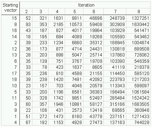
With this approach, there are four procedures that make the process easier to accomplish and the results easier to interpret:
- Rescaling
As can be seen in Figure 2, the numbers in the vectors rapidly grow from iteration to iteration in the same way that the elements in the matrix grow with the naive power method. To offset this effect, the vector can be rescaled after each iteration by multiplying by a suitable constant. Convergence to the eigenvector can be detected by monitoring the size of this correction: when it stops changing from iteration to iteration, it will be equal to the eigenvalue and the process will be finished. If this is the only adjustment made, the result will be the Frobenius eigenvector (used as Bonacich Centrality in UCINET), the eigenvector corresponding to the largest eigenvalue that would be produced by an SVD of the adjacency matrix. This operation can only be done "on the fly" after each iteration.
- Centering
Another change can be seen from iteration to iteration: a "drift" in the positive or negative direction. This can be canceled on the fly by centering the vector after each iteration which can be accomplished by subtracting the mean of the vector from its elements. Alternatively, it can be done before iterating by subtracting the row/column means from the adjacency matrix, which destroys sparsity. Both of these adjustments are equivalent to the subtraction of the means in the calculation of covariance, which is why this adjustment causes the vector to converge to the first CONVAR eigenvector.
- Normalizing
While multiplying the vector by the matrix, one may also normalize on the fly by dividing each component of the vector by the corresponding matrix row sum. Computational effort can be reduced by dividing the elements in the adjacency matrix by their corresponding row sums, so that the sum of the elements in each row becomes 1.00. In matrix notation, multiply A, the adjacency matrix, by Dr-1, a diagonal matrix of the reciprocals of the row sums of A. Because the result is a Markov matrix, we call it M. This preprocessing does not destroy sparsity.
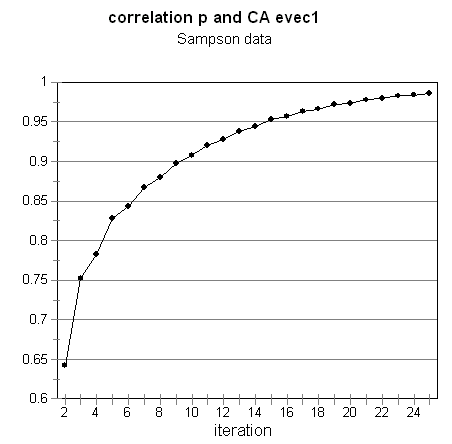
For symmetric matrices, when this kind of normalizing is done in addition to rescaling and centering, the resulting eigenvector and value will be the first non-trivial Correspondence Analysis pair (Richards & Seary, 1997). In this case, the CA eigenvectors are those of (Dr-1 A)2, which are the same as those of Dr -1 A, which is the normalized matrix being iterated. Subtracting off the row means at each step (centering) is equivalent to removing the trivial CA eigenvector. The convergence for the Sampson data is illustrated in Figure 3.
-
Figure 3.ĀĀ Convergence of random vector p to first non-trivial CA eigenvector.
If, in addition to the above adjustments, each node is given weight equal to its row sum in the matrix-vector multiplication, the resulting eigenvector will be the one corresponding to the first non-trivial positive eigenvalue of Correspondence Analysis. This eigenvector is associated with on-diagonal clustering. This is the procedure used by NEGOPY (although not to convergence).
The Power Method only provides the first eigenvector and value. To obtain subsequent pairs, the previous ones must be subtracted from the matrix before each set of iterations. This procedure, called "deflation," can also be done efficiently with sparse matrix techniques. Extra storage is needed only for each eigenvector and value. Beyond the first several eigenvector-value pairs, rounding error reduces the accuracy below acceptable limits.
The first eigenvector and value show only the mass behaviour of the system -- the behavior that is due to the proportions of interaction associated with the individual members of the network -- the marginals of A. Centering address this issue by the removal of expecteds. In geometric terms, the centering operation moves the origin of the coordinate system to the center of the space occupied by the data points. For CONVAR, this means the subtraction of row and column means from the adjacency matrix before it is subjected to the decomposition procedure. For Correspondence Analysis, the expecteds are calculated as in chi-square. The result of centering is a cleaner eigen structure that is not contaminated by leakage of information associated with the expecteds from what should be trivial eigenvectors.
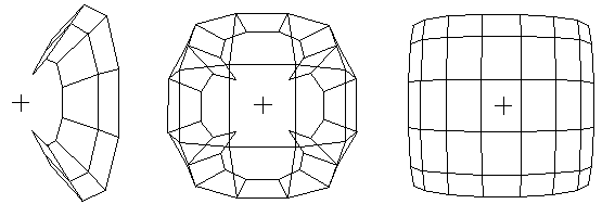
Figure 4.ĀĀ The largest two positive eigenvectors from standard
SVD, CONVAR, and CA of a 6 x 8 grid network. Origins marked "+".
When the adjacency matrix is normalized by dividing by the row sums, the largest eigenvalue becomes 1.0. Because Correspondence Analysis does this for symmetric matrices, the sum of the squared eigenvalues will be proportional to chi-squared for the adjacency matrix (when the diagonal has not been loaded). This makes it possible to see how much of the structure of the network is accounted for by each eigenvector. If a squared eigenvalue is divided by the sum of all of the squared eigenvalues, the result will vary from 0.0 to 1.0 and will tell which portion of the structure is accounted for by the corresponding eigenvector.
We can compare the effect normalizing has by considering the following equations. For Standard and CONVAR, the eigenvector components satisfy:

where "i~j" indicates the summation is over all nodes j connected to node i (Godsil, 1993, p. 261). It is easy to show that normal (CA) eigenvector components satisfy:

where "deg(i)" is the degree of node i. The important (structural) eigenvectors have ![]() > 1 and
> 1 and ![]() < 1 so that generally,
< 1 so that generally,


when the degree of node i is small. That is, for both the Standard and CONVAR, the nodes with the fewest links are pulled toward the origin and the ones with the most links pushed away. On the other hand, CA tends to push the nodes with the fewest links away from the origin and locate tightly interconnected sets of nodes near each other. These features make CA particularly useful for the identification of cohesive cliques. These effects can be seen in Figures 4 and 9.
Balancing is achieved by loading the diagonal of the
adjacency matrix before decomposition. The effect of balancing is to
shift the eigenvalues in the positive direction which effectively hides
the eigenvectors associated with what would normally be negative
eigenvalues. With Correspondence Analysis, the most effective approach
is to load the diagonal with the row sums of the adjacency matrix. With the adjacency matrix, CONCOR, or CONVAR, loading the diagonal with a sufficiently large positive constant will
have a similar effect. The next section of the paper discusses this in
further detail. There is a fair bit of confusion about the balancing
procedures we have described above. It seems that there are two major
issues:
- How to weight the diagonal
There has been uncertainty about what to do with the diagonal of the matrix since early work by Gould (1967) and Tinkler (1972) explored the possibility of using eigenvectors as tools for the structural analysis of networks of roads. Later researchers advised adding a constant to the diagonal to de-emphasize negative eigenvalues and to stabilize the matrix. Weller and Romney, in a book about Correspondence Analysis for network researchers, (1990, p. 72) argue that ". . . it is critical that the diagonal values have a large positive value," but they provide neither a justification nor an explanation of how this procedure will distort the graph's spectrum. We have studied this issue and found that in Correspondence Analysis there is a very close connection between how the diagonal is weighted and changes in the resulting set of eigenvalues. In fact, the question of how to weight the diagonal seems to be more a question of how to deal with negative eigenvalues.
- Negative eigenvalues (role vs. clique)
Most network researchers take steps to suppress or hide negative eigenvalues, which they see as problematic for a variety of reasons (e.g. Barnett, 1989). It is common to deal with the "scalar products" matrix (the transpose of a matrix multiplied by the matrix), which, since it squares the eigenvalues, hides the negative ones. Wasserman, Faust, and Glaskiewicz (1989) square the incidence matrix (they call it the "response pattern matrix"), which shifts the spectrum so that previously positive eigenvalues become larger and previously negative ones become positive (and close to zero), thus hiding the significance of the negative eigenvectors. UCINET IV calculates unbalanced Correspondence Analysis, but it does not report the signs of the eigenvalues.
Positive eigenvalues are associated with clustering of interconnected nodes and negative ones with partitioning of the network into sets of nodes that have similar patterns of connections with nodes in other sets, but few connections amongst themselves. Because CONCOR identifies structures associated with both positive and negative eigenvalues, it is useful for identifying sets of structurally equivalent nodes -- those who have similar patterns of connections with nodes in other sets. Analysts who avoid negative eigenvalues will be unable to detect structures associated with negative eigenvalues, a form of structuring that is as important as that which is associated with positive ones. This is illustrated in Figure 5, below.
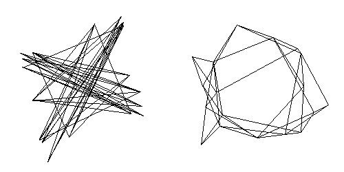
Figure 5.ĀĀ Projections on two largest eigenvectors (left) and two largest positive eigenvectors (right).
Centering, normalizing, and balancing can also be used with general
purpose eigendecomposition routines. Centering operations destroy
sparsity, but this is not an issue with routines such as the SVD
program in SPSS, which use the entire matrix anyhow. Special purpose
sparse-matrix routines, such as the Lanczos algorithm, allow the user
to define matrix vector multiplication such that the adjustments used
in the power method can be applied.
In this section we will attempt to address some practical matters.
For the large sparse arrays typical of social networks, it is not
likely that we will want a complete eigen decomposition, because most
of the important structural information is contained in the first few
dimensions. The centering, balancing, and normalizing in NEGOPY
(Richards and Rice, 1981; Richards, 1988; Richards, 1995) are done on
the fly during iterations of p' ![]() Mp, where the initial p is a random vector and M is the row-normalized adjacency matrix .
Mp, where the initial p is a random vector and M is the row-normalized adjacency matrix .
Complete eigen decomposition is O(n3), and thus impractical for large networks. What would we do with all the results? A complete decomposition would give n-1
eigenvectors and an equal number of eigenvalues. This will actually be
more numbers than were in the original data! We already know that a few
axes will probably contain most of the important information, so why
not stop after two or three dimensions? ![]() can be calculated once and used as a guide for how much of the structure has been explained.
can be calculated once and used as a guide for how much of the structure has been explained.
We have suggested that the Power Method with Deflation is a useful
way to obtain the first few eigenvectors, and for large sparse arrays
-- and two or three dimensions -- it's really not that bad. A few dozen
iterations of p' ![]() Mp gives the first non-trivial dimension F2 and its corresponding eigenvalue
Mp gives the first non-trivial dimension F2 and its corresponding eigenvalue ![]() . A few dozen more of p'
. A few dozen more of p'![]() Mp -
Mp -![]() F2
gives the second, and that may be all that is necessary to get a
reasonably informative "global" view of the structure of the network.
There are, however, more clever, faster methods of finding the first
few dimensions, such as the Lanczos method.
F2
gives the second, and that may be all that is necessary to get a
reasonably informative "global" view of the structure of the network.
There are, however, more clever, faster methods of finding the first
few dimensions, such as the Lanczos method.
We have used iteration of p'![]() Mp to extract the eigenvectors of a network. The fact that M is stochastic suggests that, in the long run, there will be a stable configuration. But in the short run, p
will be most affected by the largest (in the senses explored in the
last section) structural features. The graphs in Figure 6 show the
squared correlations of p with the first four (non-trivial) eigenvectors.
Mp to extract the eigenvectors of a network. The fact that M is stochastic suggests that, in the long run, there will be a stable configuration. But in the short run, p
will be most affected by the largest (in the senses explored in the
last section) structural features. The graphs in Figure 6 show the
squared correlations of p with the first four (non-trivial) eigenvectors.
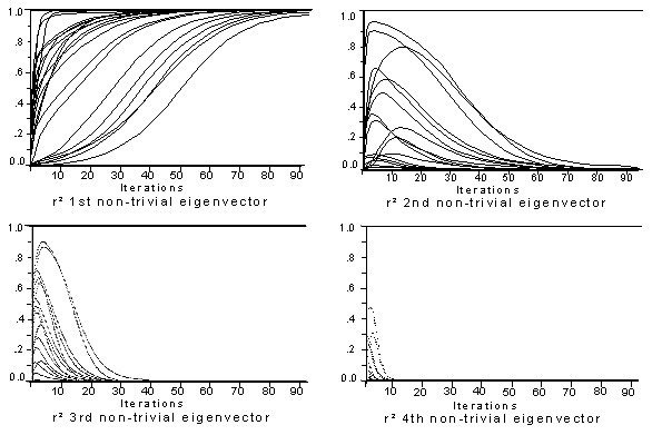
Figure 6.ĀĀ The squared correlations of p with the first four (non-trivial)
eigenvectors; 25 random starting p;
90 iterations for each.
There is a fairly wide range of variation evident in these graphs. With
some starting configurations, convergence is rapid, requiring only five
to six iterations for all but the largest eigenvector to drop out of
the picture. With other configurations, a hundred or more iterations
may be required. This variation is due to the fact that a random
starting configuration may result in a p
that points in the direction of one of the eigenvectors. If it points
in the direction of the largest one, convergence will be rapid, while
if it points in the direction of another, it will take more iterations.
In fact, if p happens to be one of the other eigenvectors, iterating may not change the position vector at all.
To make partial iteration a useful tool, we propose choosing an initial p that is orthogonal to the largest eigenvector. Since the largest eigenvector will be the positive constant determined by the matrix of expecteds, a vector containing whole number values ranging from -n/2 to n/2 (for even n) or -(n-1)/2 to (n-1)/2 (for odd n) will be suitable. This initial p will have moderately large correlations with several eigenvectors, and will converge smoothly over a moderate number of iterations, as illustrated by Fig. 7.
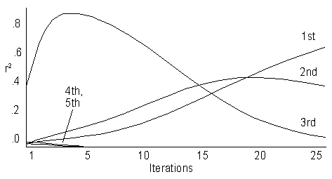
Figure 7.ĀĀ The correlations with first 5 eigenvectors over 25 iterations.
We can use this idea to devise a "divide-and-conquer" strategy for
quick analysis of the main network structures. The Spectral
Decomposition of M shows that after a few p' ![]() Mp iterations, the vector p will consist mostly of the contributions of the most "important" eigenvectors (Figure 6). In effect, we are projecting the ith iteration of M upon a single dimension. Now order p by the magnitudes of its components. Since each eigenvector induces a partition on p, we would expect to see the components of the ordered p
changing rapidly where an important eigenvector induces a partition. We
can make these partitions clearer by looking at the first difference of
ordered p, as shown in Figure 8. A more sophisticated pattern-recognition approach is used in NEGOPY.
Mp iterations, the vector p will consist mostly of the contributions of the most "important" eigenvectors (Figure 6). In effect, we are projecting the ith iteration of M upon a single dimension. Now order p by the magnitudes of its components. Since each eigenvector induces a partition on p, we would expect to see the components of the ordered p
changing rapidly where an important eigenvector induces a partition. We
can make these partitions clearer by looking at the first difference of
ordered p, as shown in Figure 8. A more sophisticated pattern-recognition approach is used in NEGOPY.
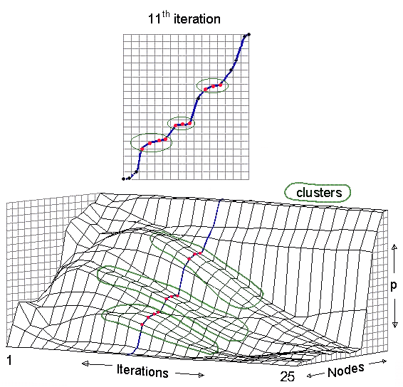
Figure 8.ĀĀ The more vertical the slope is, the farther apart the nodes are on p. Where the slope is horizontal, nodes have the same location on p. It is easy to see how clusters become visible and then disappear as the iterative process continues and more and more dimensions drop out of the picture as p converges towards the largest eigenvector. From about the 8th to the 15th iterations, three clusters are visible in the middle of the plot. By the 25th iteration, most of the nodes are clustered near the bottom.
Where the first difference of ordered p is
relatively constant, we would expect to find a cluster, and now we can
search the sparse array for the nodes defined by this cluster, and
perform any tests we wish to define "closeness," "group membership,"
and so on. Each induced partition is examined in turn. Of course, we
must subtract off the direction associated with the "trivial"
eigenvector at each step of the iteration, but this is very easy to do
even with a large sparse matrix.
We presented an introductory overview of eigen analysis methods and
their applications to network analysis. Many popular analytic
procedures used in social network analysis (eg. CONCOR, NEGOPY,
Correspondence Analysis) are at their core eigen decomposition
procedures. CA is essentially eigen decomposition of the square root of
the ![]() matrix (C - E)2 / E where E is the matrix of expected values of C;
iterated covariance produces the same result that would be obtained
with standard eigendecomposition routine of an adjacency matrix that
has had the row and column means subtracted from all its elements;
iterated correlation (CONCOR), which requires deviation scores to be
standardized by division by standard deviation, produces a binary
vector in which the components' signs are almost always the same as
those by iterated covariance. Finally, NEGOPY uses a mixture of the
eigenvectors associated with the largest positive eigenvalues of CA.
matrix (C - E)2 / E where E is the matrix of expected values of C;
iterated covariance produces the same result that would be obtained
with standard eigendecomposition routine of an adjacency matrix that
has had the row and column means subtracted from all its elements;
iterated correlation (CONCOR), which requires deviation scores to be
standardized by division by standard deviation, produces a binary
vector in which the components' signs are almost always the same as
those by iterated covariance. Finally, NEGOPY uses a mixture of the
eigenvectors associated with the largest positive eigenvalues of CA.
CONVAR, because it uses covariance rather than correlation has advantages over the closely related CONCOR: it can use sparse matrix techniques and thus can be used for very large networks; rather than the binary partitions of CONCOR, it produces eigenvectors and values and thus more information about the network's structure; because it uses only linear transformations on the adjacency matrix, it is easier to interpret than CONCOR "...whose mathematical properties are still only partially understood" (Schwartz, 1977, p. 277).
Figure 9 shows the results of a standard SVD, CONVAR, and CA of the Sampson data used earlier in the paper. All three show the coordinates associated with the two largest positive eigenvalues. The Standard analysis is not centered, so the effects of the expecteds have not been removed and their influence on the results is evident in the fact that the entire set of data points fall on one side of the origin. When the row/column means have been subtracted off, the result looks more like the one from CONVAR, which is centered by the removal of row/column means, but not normalized. For both the Standard and CONVAR, the nodes with the fewest links are pulled toward the origin and the ones with the most links pushed away. CA is centered by the removal of chi-square expecteds and normalized by the row sums which equal the number of links. With CA, the nodes with the fewest links tend to be pushed away from the origin and tightly interconnected sets of nodes tend to be located near each other, making this method particularly useful for the identification of cohesive cliques.
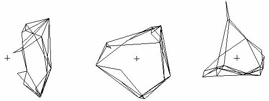
Figure 9.ĀĀ The coordinates associated with the two largest positive eigenvalues from standard
SVD, CONVAR, and CA of the Sampson data. The origins marked with "+".
We considered alternatives to complete eigendecomposition from
several perspectives: SVD of the adjacency matrix, the naive power
method which raises the matrix to successively higher powers, iterated
calculation methods (CONCOR and CONVAR), sparse matrix variant of the
power method, and partial iteration used in NEGOPY. The main advantage
of iterative approaches like the sparse power method is that they make
it possible to extract eigenvectors and values from very large
networks. Both the naive power method and iterated calculation require
the full matrix and, for asymmetric data, two copies of the matrix,
making these methods unsuitable for large networks.
We reviewed the effects of centering, normalizing, and balancing procedures carried out prior to or during the analysis. Centering moves the origin of the coordinate system to the center of the space occupied by the data points. This is done by subtraction of row and column means from the adjacency matrix before it is subjected to the decomposition procedure (CONVAR), or subtraction of the expecteds as calculated for chi-square (CA). The result of centering is a cleaner eigen structure that is not contaminated by leakage of information associated with the expecteds from what should be trivial eigenvectors. Normalizing controls for the node degree which makes the results easier to interpret and produces better clustering. Balancing can be used to hide or suppress the eigenvectors associated with negative eigenvalues. This makes on-diagonal clusters visible and hides off-diagonal clusters or blocks.
Finally, we examined partial decomposition strategies and showed how they make it possible to extract information about the structure of a network in an efficient and practical manner. For example, using partial iteration, NEGOPY is able to analyze networks with up to 3,200 nodes and 25,000 links in a program that runs in under 550K in DOS.
Acton, F. (1990). Numerical Methods That Work. Harper and Row.
Barnett, G.A. (1989). Approaches to non-Euclidean network analysis. In M. Kochen (ed.), Small World, pp. 349-372. Norwood, NJ: Ablex.
Gould, P. (1967). The Geographical Interpretation of Eigenvalues. Institute of British Geographers Transactions, 42: 53-85.
Greenacre, M. (1984). Theory and Application of Correspondence Analysis. Academic Press.
Hoffman, D., Franke, G. (1986). Correspondence Analysis: Graphical Representation of Categorical Data in Marketing Research. J. Market Research 23: 213-227.
Parlett, B. (1979). The Lanczos algorithm with selective orthogonalization. Mathematics of Computation, 33: 145, 217-238.
Richards, W.D. (1988). NEGOPY for Microcomputers. Connections (the Bulletin of the International Network for Social Network Analysis), Vol. XI, No. 3.
Richards, W.D. (1995). NEGOPY 4.30 Manual and User's Guide. School of Communication, Simon Fraser University, Burnaby, BC, Canada.
Richards, W.D. and R. Rice. (1981). The NEGOPY Network Analysis Program. Social Networks, 3:3, pp. 215.
Richards, W.D. and Seary, A.J. (1997). "Convergence analysis of communication networks" in Barnett, G.A. (ed.), Advances in Communication Sciences, Vol. 15, pp. 141-189. Norwood, NJ: Ablex.
Schwartz, J.E. (1977). An examination of CONCOR and related methods for blocking sociometric data, in Heise, D.R. (ed). Sociological Methodology 1977, pp. 255-282. San Francisco: Jossey-Bass.
Tinkler, K. (1972). The Physical Interpretation of Eigenfunctions of Dichotomous Matrices. Inst. Br. Geog. Trans.. 55, 17-46.
Wasserman, S., Faust, K., and Glaskiewicz, J. (1989). Correspondence and canonical analysis of relational data. J. Mathematical Sociology. 1:1, 11-64.
Weller, S., Romney, A. (1990). Metric Scaling: Correspondence Analysis. Beverly Hills: Sage.